Finite volume
From CFD-Wiki
Contents |
Discretisation Schemes for convective terms in General Transport Equation. Finite-Volume Formulation, structured grids
Introduction
Here is describing the discretization schemes of the convective terms in the finite-volume equations. The accuracy, numerical stability and the boundness of the solution depends on the numerical scheme used for these terms. The central issue is the specification of an appropriate relationship between the convected variable, stored at the cell centre and its value at each of the cell faces.
Basic Equations of CFD
All the conservation equations can be written in the same generic differential form:
|
| (1) |
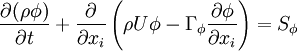
Equation (1) is integrated over a control volume and the following discretised equation for  is produced:
|
| (2) |

whereis the source term for the control volume
, and $J_{f}$ and $D_{f}$ represent, respectively, the convective and diffusive fluxes of $\phi$ across the control-volume face $f$ ($f=h,l,n,s,e,w$) The convective fluxes through the cell faces are calculated as:
|
| (1) |

where $C_{f}$ is the mass flow rate across the cell face $f$. The convected variable $\phi_{f}$ associated with this mass flow rate is usually stored at the cell centres, and thus some form of interpolation assumption must be made in order to determine its value at each cell face. The interpolation procedure employed for this operation is the subject of the various schemes proposed in the literature and the accuracy, stability and boundedness of the solution depends on the procedure used.
In general, the value of $\phi_{f}$ can be explicity formulated in terms of its neighbouring nodal values by a functional relationship of the form:
|
| (1) |
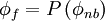
where $\phi_{nb}$ denotes the neighbouring-node $\phi$ values.
Combining equations (\ref{eq3}) through (\ref{eq4a}), the discretised equation becomes:
|
| (1) |
![\left\{ D_{h} + C_{h} \left[ P \left( \phi_{nb} \right) \right]_{h} \right\} -
\left\{ D_{l} + C_{l} \left[ P \left( \phi_{nb} \right) \right]_{l} \right\} +
\left\{ D_{n} + C_{n} \left[ P \left( \phi_{nb} \right) \right]_{n} \right\} -
\left\{ D_{s} + C_{s} \left[ P \left( \phi_{nb} \right) \right]_{s} \right\} +
\left\{ D_{e} + C_{e} \left[ P \left( \phi_{nb} \right) \right]_{e} \right\} -
\left\{ D_{w} + C_{w} \left[ P \left( \phi_{nb} \right) \right]_{w} \right\} = S_{p}](/W/images/math/8/a/7/8a710ce35af1c5c95cf741524ecd18f6.png)
Convection Schemes
All the convection schemes involve a stencil of cells in which the values of $\phi$ will be used to construct the face value $\phi_{f}$
\begin{figure}[h] \centering \includegraphics{D:/TeXWorkPlace/Wikki_Article/Picture_01.jpg} \caption{Stensil of cells}
\label{fig:Picture_01} \end{figure}
Where flow is from left to right, and $f$ is the face in question.
Basic Discretisation schemes
Central Differencing Scheme (CDS)
The most natural assumption for the cell-face value of the convected variable $\phi_{f}$ would appear to be the CDS, which calculates the cell-face value from:
|
| (1) |
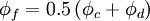
This scheme is 2nd-order accurate, but is unbounded so that unphysical oscillations appear in regions of strong convection and also in the presence of discontinuities such as shocks. The CDS may be used directly in very low Reynolds-number flows where diffusive effects dominate over convection.
Upwind Differencing Scheme (UDS)
The UDS assumes that the convected variable at the cell fase $f$ is the same as the upwind cell-centre value:
|
| (1) |

The UDS is unconditionally bounded and highly stable, but as noted earlier it is only 1st-order accurate in terms of truncation error and may produce severe numerical diffusion. The scheme is therefore highly diffusive when the flow direction is skewed relative to the grid lines.