Gauss-Seidel method
From CFD-Wiki
(Added an example calculation (finally)) |
|||
| (7 intermediate revisions not shown) | |||
| Line 1: | Line 1: | ||
| - | + | The '''Gauss-Seidel method''' is a technique used to solve a linear system of equations. The method is named after the German mathematician [http://en.wikipedia.org/wiki/Carl_Friedrich_Gauss Carl Friedrich Gauss] and [http://en.wikipedia.org/wiki/Philipp_Ludwig_von_Seidel Philipp Ludwig von Seidel]. The method is similar to the [[Jacobi method]] and in the same way strict or irreducible diagonal dominance of the system is sufficient to ensure convergence, meaning the method will work. | |
| - | We seek the solution to set of linear equations: <br> | + | We seek the solution to a set of linear equations: <br> |
:<math> A \phi = b </math> <br> | :<math> A \phi = b </math> <br> | ||
| Line 11: | Line 11: | ||
</math> | </math> | ||
| - | where <math>D</math>, <math>L</math>, and <math>U</math> represent the diagonal, lower triangular, and upper triangular parts of the coefficient matrix <math>A</math> | + | where <math>A=D-L-U</math> and <math>D</math>, <math>L</math>, and <math>U</math> represent the diagonal, lower triangular, and upper triangular parts of the coefficient matrix <math>A</math>. <math>k</math> is the iteration count. This matrix expression is mainly of academic interest, and is not used to program the method. Rather, an element-based approach is used: |
:<math> | :<math> | ||
| Line 20: | Line 20: | ||
== Algorithm == | == Algorithm == | ||
| - | : | + | : Choose an initial guess <math>\phi^{0}</math> <br> |
: for k := 1 step 1 until convergence do <br> | : for k := 1 step 1 until convergence do <br> | ||
:: for i := 1 step until n do <br> | :: for i := 1 step until n do <br> | ||
| Line 34: | Line 34: | ||
:: check if convergence is reached | :: check if convergence is reached | ||
: end (k-loop) | : end (k-loop) | ||
| + | |||
| + | ==Convergence== | ||
| + | |||
| + | The method will always converge if the matrix ''A'' is strictly or irreducibly diagonally dominant. Strict row diagonal dominance means that for each row, the absolute value of the diagonal term is greater than the sum of absolute values of other terms: | ||
| + | |||
| + | :<math>\left | a_{ii} \right | > \sum_{i \ne j} {\left | a_{ij} \right |} </math> | ||
| + | |||
| + | The Gauss-Seidel method sometimes converges even if this condition is not satisfied. It is necessary, however, that the diagonal terms in the matrix are greater (in magnitude) than the other terms. | ||
== Example Calculation == | == Example Calculation == | ||
In some cases, we need not even explicitly represent the matrix we are solving. Consider the simple heat equation problem | In some cases, we need not even explicitly represent the matrix we are solving. Consider the simple heat equation problem | ||
| - | :<math>\nabla^2 T = 0</math> | + | :<math>\nabla^2 T(x) = 0,\ x\in [0,1]</math> |
| - | + | subject to the boundary conditions <math>T(0)=0</math> and <math>T(1)=1</math>. The exact solution to this problem is <math>T(x)=x</math>. The standard second-order finite difference discretization is | |
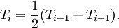
:<math> T_{i-1}-2T_i+T_{i+1} = 0,</math> | :<math> T_{i-1}-2T_i+T_{i+1} = 0,</math> | ||
| Line 84: | Line 92: | ||
:<math> T_i = \frac{1}{2}(T_{i-1}+T_{i+1}).</math> | :<math> T_i = \frac{1}{2}(T_{i-1}+T_{i+1}).</math> | ||
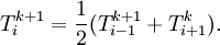
| - | Then, stepping through the solution vector from <math>i=2</math> to <math>i=n-1</math>, we can compute the next iterate from the two surrounding values. Note that (in this scheme), <math>T_{i+1}</math> is from the previous iteration, while <math>T_{i-1}</math> is from the current iteration. | + | Then, stepping through the solution vector from <math>i=2</math> to <math>i=n-1</math>, we can compute the next iterate from the two surrounding values. Note that (in this scheme), <math>T_{i+1}</math> is from the previous iteration, while <math>T_{i-1}</math> is from the current iteration: |
| + | |||
| + | :<math> T_i^{k+1} = \frac{1}{2}(T_{i-1}^{k+1}+T_{i+1}^k).</math> | ||
| + | |||
| + | The following table gives the results of 10 iterations with 5 nodes (3 interior and 2 boundary) as well as <math>L_2</math> norm error. | ||
{| align=center border=1 | {| align=center border=1 | ||
| - | ! Iteration !! | + | |+ Gauss-Seidel Solution (i=2,3,4) |
| + | ! Iteration !! <math>T_1</math> !! <math>T_2</math> !! <math>T_3</math> !! <math>T_4</math> !! <math>T_5</math> !! <math>L_2</math> error | ||
|- | |- | ||
| 0 | | 0 | ||
| Line 177: | Line 190: | ||
| 1.4648E-03 | | 1.4648E-03 | ||
|} | |} | ||
| + | |||
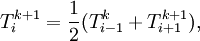
| + | In this situation, the direction that we "sweep" is important - if we step though the solution vector in the opposite direction, the solution moves away from the chosen initial condition (zero everywhere in the interior) more quickly. The iteration is defined by | ||
| + | |||
| + | :<math> T_i^{k+1} = \frac{1}{2}(T_{i-1}^{k}+T_{i+1}^{k+1}),</math> | ||
| + | |||
| + | and this gives us (slightly) faster convergence, as shown in the table below. | ||
| + | |||
| + | {| align=center border=1 | ||
| + | |+ Gauss-Seidel Solution (i=4,3,2) | ||
| + | ! Iteration !! <math>T_1</math> !! <math>T_2</math> !! <math>T_3</math> !! <math>T_4</math> !! <math>T_5</math> !! <math>L_2</math> error | ||
| + | |- | ||
| + | | 0 | ||
| + | | 0.0000E+00 | ||
| + | | 0.0000E+00 | ||
| + | | 0.0000E+00 | ||
| + | | 0.0000E+00 | ||
| + | | 1.0000E+00 | ||
| + | | 1.0000E+00 | ||
| + | |- | ||
| + | | 1 | ||
| + | | 0.0000E+00 | ||
| + | | 1.2500E-01 | ||
| + | | 2.5000E-01 | ||
| + | | 5.0000E-01 | ||
| + | | 1.0000E+00 | ||
| + | | 3.7500E-01 | ||
| + | |- | ||
| + | | 2 | ||
| + | | 0.0000E+00 | ||
| + | | 1.8750E-01 | ||
| + | | 3.7500E-01 | ||
| + | | 6.2500E-01 | ||
| + | | 1.0000E+00 | ||
| + | | 1.8750E-01 | ||
| + | |- | ||
| + | | 3 | ||
| + | | 0.0000E+00 | ||
| + | | 2.1875E-01 | ||
| + | | 4.3750E-01 | ||
| + | | 6.8750E-01 | ||
| + | | 1.0000E+00 | ||
| + | | 9.3750E-02 | ||
| + | |- | ||
| + | | 4 | ||
| + | | 0.0000E+00 | ||
| + | | 2.3438E-01 | ||
| + | | 4.6875E-01 | ||
| + | | 7.1875E-01 | ||
| + | | 1.0000E+00 | ||
| + | | 4.6875E-02 | ||
| + | |- | ||
| + | | 5 | ||
| + | | 0.0000E+00 | ||
| + | | 2.4219E-01 | ||
| + | | 4.8438E-01 | ||
| + | | 7.3438E-01 | ||
| + | | 1.0000E+00 | ||
| + | | 2.3438E-02 | ||
| + | |- | ||
| + | | 6 | ||
| + | | 0.0000E+00 | ||
| + | | 2.4609E-01 | ||
| + | | 4.9219E-01 | ||
| + | | 7.4219E-01 | ||
| + | | 1.0000E+00 | ||
| + | | 1.1719E-02 | ||
| + | |- | ||
| + | | 7 | ||
| + | | 0.0000E+00 | ||
| + | | 2.4805E-01 | ||
| + | | 4.9609E-01 | ||
| + | | 7.4609E-01 | ||
| + | | 1.0000E+00 | ||
| + | | 5.8594E-03 | ||
| + | |- | ||
| + | | 8 | ||
| + | | 0.0000E+00 | ||
| + | | 2.4902E-01 | ||
| + | | 4.9805E-01 | ||
| + | | 7.4805E-01 | ||
| + | | 1.0000E+00 | ||
| + | | 2.9297E-03 | ||
| + | |- | ||
| + | | 9 | ||
| + | | 0.0000E+00 | ||
| + | | 2.4951E-01 | ||
| + | | 4.9902E-01 | ||
| + | | 7.4902E-01 | ||
| + | | 1.0000E+00 | ||
| + | | 1.4648E-03 | ||
| + | |- | ||
| + | | 10 | ||
| + | | 0.0000E+00 | ||
| + | | 2.4976E-01 | ||
| + | | 4.9951E-01 | ||
| + | | 7.4951E-01 | ||
| + | | 1.0000E+00 | ||
| + | | 7.3242E-04 | ||
| + | |} | ||
| + | |||
| + | For this toy example, there is not large penalty for choosing the wrong sweep direction. For some of the more complicated variants of Gauss-Seidel, there is a substantial penalty - the sweep direction determines (in a vague sense) the direction in which information travels. | ||
| + | |||
| + | ==External links== | ||
| + | |||
| + | *[http://www.math-linux.com/spip.php?article48 Gauss-Seidel from www.math-linux.com] | ||
| + | *[http://mathworld.wolfram.com/Gauss-SeidelMethod.html Gauss-Seidel from MathWorld] | ||
| + | *[http://en.wikipedia.org/wiki/Gauss_seidel Gauss-Seidel from Wikipedia] | ||
Latest revision as of 09:15, 3 January 2012
The Gauss-Seidel method is a technique used to solve a linear system of equations. The method is named after the German mathematician Carl Friedrich Gauss and Philipp Ludwig von Seidel. The method is similar to the Jacobi method and in the same way strict or irreducible diagonal dominance of the system is sufficient to ensure convergence, meaning the method will work.
We seek the solution to a set of linear equations:

In matrix terms, the the Gauss-Seidel iteration can be expressed as
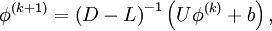
where 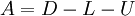 and
and  ,
,  , and
, and  represent the diagonal, lower triangular, and upper triangular parts of the coefficient matrix
  .
.  is the iteration count. This matrix expression is mainly of academic interest, and is not used to program the method. Rather, an element-based approach is used:
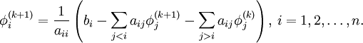
Note that the computation of  uses only those elements of
  that have already been computed and only those elements of
  that have yet to be advanced to iteration
  . This means that no additional storage is required, and the computation can be done in place ( replaces ). While this might seem like a rather minor concern, for large systems it is unlikely that every iteration can be stored. Thus, unlike the Jacobi method, we do not have to do any vector copying should we wish to use only one storage vector. The iteration is generally continued until the changes made by an iteration are below some tolerance.
Contents |
Algorithm
- Choose an initial guess

- for k := 1 step 1 until convergence do
- for i := 1 step until n do
-

- for j := 1 step until i-1 do
-
- end (j-loop)
- for j := i+1 step until n do
-
- end (j-loop)
-
-
- end (i-loop)
- check if convergence is reached
- for i := 1 step until n do
- end (k-loop)
Convergence
The method will always converge if the matrix A is strictly or irreducibly diagonally dominant. Strict row diagonal dominance means that for each row, the absolute value of the diagonal term is greater than the sum of absolute values of other terms:
The Gauss-Seidel method sometimes converges even if this condition is not satisfied. It is necessary, however, that the diagonal terms in the matrix are greater (in magnitude) than the other terms.
Example Calculation
In some cases, we need not even explicitly represent the matrix we are solving. Consider the simple heat equation problem
![\nabla^2 T(x) = 0,\ x\in [0,1]](/W/images/math/6/8/1/681af3c6083368314f689c744b5b198c.png)
subject to the boundary conditions  and
and  . The exact solution to this problem is
  . The standard second-order finite difference discretization is
where  is the (discrete) solution available at uniformly spaced nodes. In matrix terms, this can be written as
![\left[
\begin{matrix}
{1 } & {0 } & {0 } & \cdot & \cdot & { 0 } \\
{1 } & {-2 } & {1 } & { } & { } & \cdot \\
{ 0 } & {1 } & {-2 } & { 1 } & { } & \cdot \\
{ } & { } & \cdot & \cdot & \cdot & \cdot \\
{ } & { } & { } & {1 } & {-2 } & {1 }\\
{ 0 } & \cdot & \cdot & { 0 } & { 0 } & {1 }\\
\end{matrix}
\right]
\left[
\begin{matrix}
{T_1 } \\
{T_2 } \\
{T_3 } \\
\cdot \\
{T_{n-1} } \\
{T_n } \\
\end{matrix}
\right]
=
\left[
\begin{matrix}
{0} \\
{0} \\
{0} \\
\cdot \\
{0} \\
{1} \\
\end{matrix}
\right].](/W/images/math/0/9/6/0969684693ca0c618b2b9ba12bd8695d.png)
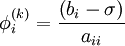
However, for any given for  , we can write
Then, stepping through the solution vector from  to
to  , we can compute the next iterate from the two surrounding values. Note that (in this scheme),
  is from the previous iteration, while
  is from the current iteration:
The following table gives the results of 10 iterations with 5 nodes (3 interior and 2 boundary) as well as  norm error.
| Iteration |  |  |  |  |  | error
|
|---|---|---|---|---|---|---|
| 0 | 0.0000E+00 | 0.0000E+00 | 0.0000E+00 | 0.0000E+00 | 1.0000E+00 | 1.0000E+00 |
| 1 | 0.0000E+00 | 0.0000E+00 | 0.0000E+00 | 5.0000E-01 | 1.0000E+00 | 6.1237E-01 |
| 2 | 0.0000E+00 | 0.0000E+00 | 2.5000E-01 | 6.2500E-01 | 1.0000E+00 | 3.7500E-01 |
| 3 | 0.0000E+00 | 1.2500E-01 | 3.7500E-01 | 6.8750E-01 | 1.0000E+00 | 1.8750E-01 |
| 4 | 0.0000E+00 | 1.8750E-01 | 4.3750E-01 | 7.1875E-01 | 1.0000E+00 | 9.3750E-02 |
| 5 | 0.0000E+00 | 2.1875E-01 | 4.6875E-01 | 7.3438E-01 | 1.0000E+00 | 4.6875E-02 |
| 6 | 0.0000E+00 | 2.3438E-01 | 4.8438E-01 | 7.4219E-01 | 1.0000E+00 | 2.3438E-02 |
| 7 | 0.0000E+00 | 2.4219E-01 | 4.9219E-01 | 7.4609E-01 | 1.0000E+00 | 1.1719E-02 |
| 8 | 0.0000E+00 | 2.4609E-01 | 4.9609E-01 | 7.4805E-01 | 1.0000E+00 | 5.8594E-03 |
| 9 | 0.0000E+00 | 2.4805E-01 | 4.9805E-01 | 7.4902E-01 | 1.0000E+00 | 2.9297E-03 |
| 10 | 0.0000E+00 | 2.4902E-01 | 4.9902E-01 | 7.4951E-01 | 1.0000E+00 | 1.4648E-03 |
In this situation, the direction that we "sweep" is important - if we step though the solution vector in the opposite direction, the solution moves away from the chosen initial condition (zero everywhere in the interior) more quickly. The iteration is defined by
and this gives us (slightly) faster convergence, as shown in the table below.
| Iteration | | | | | | error
|
|---|---|---|---|---|---|---|
| 0 | 0.0000E+00 | 0.0000E+00 | 0.0000E+00 | 0.0000E+00 | 1.0000E+00 | 1.0000E+00 |
| 1 | 0.0000E+00 | 1.2500E-01 | 2.5000E-01 | 5.0000E-01 | 1.0000E+00 | 3.7500E-01 |
| 2 | 0.0000E+00 | 1.8750E-01 | 3.7500E-01 | 6.2500E-01 | 1.0000E+00 | 1.8750E-01 |
| 3 | 0.0000E+00 | 2.1875E-01 | 4.3750E-01 | 6.8750E-01 | 1.0000E+00 | 9.3750E-02 |
| 4 | 0.0000E+00 | 2.3438E-01 | 4.6875E-01 | 7.1875E-01 | 1.0000E+00 | 4.6875E-02 |
| 5 | 0.0000E+00 | 2.4219E-01 | 4.8438E-01 | 7.3438E-01 | 1.0000E+00 | 2.3438E-02 |
| 6 | 0.0000E+00 | 2.4609E-01 | 4.9219E-01 | 7.4219E-01 | 1.0000E+00 | 1.1719E-02 |
| 7 | 0.0000E+00 | 2.4805E-01 | 4.9609E-01 | 7.4609E-01 | 1.0000E+00 | 5.8594E-03 |
| 8 | 0.0000E+00 | 2.4902E-01 | 4.9805E-01 | 7.4805E-01 | 1.0000E+00 | 2.9297E-03 |
| 9 | 0.0000E+00 | 2.4951E-01 | 4.9902E-01 | 7.4902E-01 | 1.0000E+00 | 1.4648E-03 |
| 10 | 0.0000E+00 | 2.4976E-01 | 4.9951E-01 | 7.4951E-01 | 1.0000E+00 | 7.3242E-04 |
For this toy example, there is not large penalty for choosing the wrong sweep direction. For some of the more complicated variants of Gauss-Seidel, there is a substantial penalty - the sweep direction determines (in a vague sense) the direction in which information travels.