Introduction to turbulence

From CFD-Wiki

(Difference between revisions)

Revision as of 09:13, 14 September 2005

What is Turbulence?

Turbulence is that state of fluid motion which is characterized by apparently random and chaotic three-dimensional vorticity. When turbulence is present, it usually dominates all other flow phenomena and results in increased energy dissipation, mixing, heat transfer, and drag.

For a long time scientists were not really sure in which sense turbulence is 'random', but they were pretty sure it was. Like any one who is trained in physics, we believe the flows we see around us must be the solution to some set of equations which govern. (This is after all what mechanics is about- writing equations to describe and predict the world around us) But because of the nature of the turbulence, it wasn't clear whether the equations themselves had some hidden randomness, or just the solutions. And if the latter, was it something the equations did to them, or a consequence of the intial conditions

Why Study Turbulence?

There really are the two reasons for studying turbulence- engineering and physics! And they are not necessarily complementary, atleast in the short run.

Certainly a case can be made that we don't know enough about the turbulence to even start to consider engineering problems. To begin with, we always have fewer equations that unknowns in any attempt to predict anything other than the instantaneous motions. This is the famous turbulence closure problem.

Of course, closure is not a problem when performing a so called DNS simulation (Direct Numerical Simulations) in which we numerically produce the instantaneous motions in a computer using the exact equations governing the fluid. Unfortunately we won't be able to perform such simulations for real engineering problems until atleast a few hundred generations of computers have come and gone. And this wo't really help us too much, since even when we now perform a DNS simulation of a really simple flow, we are already overwhelmed by the amount of data and its apparent random behaviour. This is because without some kind of theory, we have no criteria for selecting from it in a single lifetime what is important.

The engineer's counter argument to the scientist's lament above is:

airplanes must fly,
weather must be forecast,
sewage and water management systems must be built
society needs ever more energy-efficient hardware and gadgets.

Thus the engineer argues, no matter the inadequate state of our knowledge, we have the responsibilty as engineers to do the best we can with what we have. Who, considering the needs, could seriously argue with this? Almost incredibly - some physicists do!

It seems evindent then that there must be at least two levels of assault on turbulence. At one level, the very nature of turbulence must be explored. At the other level, our current state of knowledge- however inadequate it might be- must be stretched to provide engineering solutions to real problems.

The cost of our ignorance

It is difficult to place a price tag on the cost of our limited understanding of turbulence, but it requires no imagination at all to realize that it must be enormous. Try to estimate, for example, the aggregate cost to society of our limited turbulence prediction abilities which result in inadequate weather-forecasts alone. Or try to place a value on the increased cost to the consumer need of the designer of virtually every fluid-thermal system-from heat exchangers to hypersonic planes- to depend on empiricism and experimentation, with the resulting need for abundant safety factors and non-optimal performance by all but the crudest measures.Or consider the frustration to engineers and cost to management of the never-ending need for 'code-validation' experiments every time a new class of flows is encounteredor major design change is contemplated. The whole idea of 'codes' in the first place was to be able to evaluate designs wihtout having to do experiments or build prototypes.

What do we really know for sure?

Turbulence is a subject on which still studies are going on. We really don't know a whole lot for sure about turbulence. And worse, we even disagree about what we think we know! There are indeed some things some researchers think we understand pretty well - like for example the kolmogorov similarity theory for the dissipative scales and the Law of the Wall for wall-bounded flows. These are based on assumptions and logical constructions about how we believe turbulence behaves in the limit of infinite Reynolds number. But even these ideas have never been tested in controlled laboratory ecperiments in the limits of high Reynolds number, because no one has ever had the large scale facilities required to do so.

It seems to be a characteristic of humans(and contrary to popular beleif, scientists and engineers are indeed human) that we tend to accept ideas which have been around a while as fact, instead of just working hypotheses that are still waiting to be tested. One can reasonably argue that the acceptance of most ideas in turbulence is perhaps more due to the time lapsed since they were proposed and found to be in resonable agreement with limited data base, than that they have been subjected to experimental tests over the range of their assumed validity. Thus it might be wise to view most 'established' laws and theories of turbulence as more like religious creeds than matters of fact.

The whole situation is a bit analogous to the old idea that the sun and stars revolved around the earth - it was a fine idea, and even good today for navigational purposes. The only problem was that one day someone (Copernicus, Brahe and Galileo among them) looked up and realized it wasn't true. So it may be with a lot of what we believe today to be true about turbulence - some day you may be the one to look at evidence in a new way and decide that things we thought to be true are wrong.

The Reynolds Averaged Equations and the Turbulence Closure Problem

1. The Equations Governing the Instantaneous Fluid Motions

All fluid motions, whether turbulent or not, are governed by the dynamical equations for a fluid. These can be written using Cartesian tensor notation as:

$\rho\left[\frac{\partial \tilde{u_i}}{\partial t}+\tilde{u_j}\frac{\partial \tilde{u_i}}{\partial x_j}\right] = -\frac{\partial \tilde{p}}{\partial x_i}+\frac{\partial \tilde{T_{ij}}^{(v)}}{\partial x_j}$

(2.1)

$\left[\frac{\partial \tilde{\rho}}{\partial t}+\tilde{u_j}\frac{\partial \tilde{\rho}}{\partial x_j}\right]+ \tilde{\rho}\frac{\partial \tilde{u_j}}{\partial x_j}= 0$

(2.2)

where $\tilde{u_i}(\vec{x},t)$ represents the i-the component of the fluid velocity at a point in space, $[\vec{x}]_i=x_i$ , and time,t. Also $\tilde{p}(\vec{x},t)$ represents the static pressure, $\tilde{T_{ij}}^{(v)}(\vec{x},t)$ , the viscous(or deviatoric) stresses, and $\tilde\rho$ the fluid density. The tilde over the symbol indicates that an instantaneous quantity is being considered. Also the Einstein summation convention has been employed[1].

In equation 2.1, the subscript i is a free index which can take on the values 1,2 and 3. Thus equation 2.1 is in reality three separate equations. These three equations are just Newton's second law written for a continuum in a spatial(or Eulerian) reference frame. Together they relate the rate of change of momentum per unit mass $(\rho{u_i})$ ,a vector quantity, to the contact and body forces.

Equation 2.2 is the equation for mass conservation in the absence of sources(or sinks) of mass. Almost all flows considered in this material will be incompressible, which implies that derivative of the density following the fluid material[the term in brackets] is zero. Thus for incompressible flows, the mass conservation equation reduces to:

$\frac{D \tilde{\rho}}{Dt}=\frac{\partial \tilde{\rho}}{\partial t}+\tilde{u_j}\frac{\partial \tilde{\rho}}{\partial x_j}= 0$

(2.3)

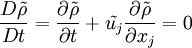
From equation 2.2 it follows that for incompressible flows,

$\frac{\partial \tilde{u_i}}{\partial x_j}= 0$

(2.4)

The viscous stresses(the stress minus the mean normal stress) are represented by the tensor $\tilde{T_{ij}}^{(v)}$ . From its definition, $\tilde{T_{kk}}^{(v)}$ =0. In many flows of interest, the fluid behaves as a Newtonian fluid in which the viscous stress can be related to the fluid motion by a constitutive relation of the form.

$\tilde{T_{ij}}^{(v)}= 2\mu[\tilde{s_{ij}}-\frac{1}{3}\tilde{s_{kk}}\delta_{ij}]$

(2.5)

The viscosity, $\mu$ , is a property of the fluid that can be measured in an independent experiment. $\tilde s_{ij}$ is the instantaneous strain rate tensor defoned by

$\tilde{s_{ij}}= \frac{1}{2}\left[\frac{\partial \tilde u_i}{\partial x_j}+\frac{\partial \tilde u_j}{\partial x_i}\right]$

(2.6)

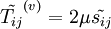
From its definition, $\tilde s_{kk}=\frac{\partial \tilde u_k}{\partial x_k}$ . If the flow is incompressible, $\tilde s_{kk}=0$ and the Newtonian constitutive equation reduces to

$\tilde{T_{ij}}^{(v)}= 2\mu\tilde{s_{ij}}$

(2.7)

Throughout this material, unless explicitly stated otherwise, the density $\tilde\rho=\rho$ and the viscosity $\mu$ will be assumed constant. With these assumptions, the instantaneous momentum equations for a Newtonian Fluid reduce to:

$\left[\frac{\partial \tilde{u_i}}{\partial t}+\tilde{u_j}\frac{\partial \tilde{u_i}}{\partial x_j}\right] = -\frac {1}{\tilde\rho}\frac{\partial \tilde{p}}{\partial x_i}+\nu\frac{\partial^2 {\tilde{u_i}}}{\partial x_j^2}$

(2.8)

where the kinematic viscosity, $\nu$ , has been defined as:

$\nu\equiv\frac{\mu}{\rho}$

(2.9)

Note that since the density is assumed conastant, the tilde is no longer necessary.

Sometimes it will be more instructive and convenient to not explicitly include incompressibilty in the stress term, but to refer to the incompressible momentum equation in the following form:

$\rho\left[\frac{\partial \tilde{u_i}}{\partial t}+\tilde{u_j}\frac{\partial \tilde{u_i}}{\partial x_j}\right] = -\frac{\partial \tilde{p}}{\partial x_i}+\frac{\partial \tilde{T_{ij}}^{(v)}}{\partial x_j}$

(2.10)

This form has the advantage that it is easier to keep track of the exact role of the viscous stresses.

2. Equations for the Average Velocity

Credits

This text was based on "Introduction to Turbulence" by Professor William K.George, Chalmers University of Technology, Sweden.

@@ Line 35: / Line 35: @@
 The whole situation is a bit analogous to the old idea that the sun and stars revolved around the earth - it was a fine idea, and even good today for navigational purposes. The only problem was that one day someone (Copernicus, Brahe and Galileo among them) looked up and realized it wasn't true. So it may be with a lot of what we believe today to be true about turbulence - some day you may be the one to look at evidence in a new way and decide that things we thought to be true are wrong.
+==The Reynolds Averaged Equations and the Turbulence Closure Problem==
+'''1. The Equations Governing the Instantaneous Fluid Motions'''
+All fluid motions, whether turbulent or not, are governed by the dynamical equations for a fluid. These can be written using Cartesian tensor notation as:
+<table width="100%">
+<tr><td>
+:<math>
+\rho\left[\frac{\partial \tilde{u_i}}{\partial t}+\tilde{u_j}\frac{\partial \tilde{u_i}}{\partial x_j}\right] = -\frac{\partial \tilde{p}}{\partial x_i}+\frac{\partial \tilde{T_{ij}}^{(v)}}{\partial x_j}</math>
+</td><td width="5%">(2.1)</td></tr></table>
+<table width="100%">
+<tr><td>
+:<math>
+\left[\frac{\partial \tilde{\rho}}{\partial t}+\tilde{u_j}\frac{\partial \tilde{\rho}}{\partial x_j}\right]+ \tilde{\rho}\frac{\partial \tilde{u_j}}{\partial x_j}= 0 </math>
+</td><td width="5%">(2.2)</td></tr></table>
+where <math>\tilde{u_i}(\vec{x},t)</math> represents the i-the component of the fluid velocity at a point in space,<math>[\vec{x}]_i=x_i</math>, and time,t. Also
+<math>\tilde{p}(\vec{x},t)</math> represents the static pressure, <math>\tilde{T_{ij}}^{(v)}(\vec{x},t)</math>, the viscous(or deviatoric) stresses, and <math>\tilde\rho</math> the fluid density. The tilde over the symbol indicates that an instantaneous quantity is being considered. Also the Einstein summation convention has been employed[1].
+In equation 2.1, the subscript i is a free index which can take on the values 1,2 and 3. Thus equation 2.1 is in reality three separate equations. These three equations are just Newton's second law written for a continuum in a spatial(or Eulerian) reference frame. Together they relate the rate of change of momentum per unit mass <math>(\rho{u_i})</math>,a vector quantity, to the contact and body forces.
+Equation 2.2 is the equation for mass conservation in the absence of sources(or sinks) of mass. Almost all flows considered in this material will be incompressible, which implies that derivative of the density following the fluid material[the term in brackets] is zero. Thus for incompressible flows, the mass conservation equation reduces to:
+<table width="100%">
+<tr><td>
+:<math>
+\frac{D \tilde{\rho}}{Dt}=\frac{\partial \tilde{\rho}}{\partial t}+\tilde{u_j}\frac{\partial \tilde{\rho}}{\partial x_j}= 0</math>
+</td><td width="5%">(2.3)</td></tr></table>
+From equation 2.2 it follows that for incompressible flows,
+<table width="100%">
+<tr><td>
+:<math>
+\frac{\partial \tilde{u_i}}{\partial x_j}= 0</math>
+</td><td width="5%">(2.4)</td></tr></table>
+The viscous stresses(the stress minus the mean normal stress) are represented by the tensor<math>\tilde{T_{ij}}^{(v)}</math>. From its definition,<math>\tilde{T_{kk}}^{(v)}</math>=0. In many flows of interest, the fluid behaves as a Newtonian fluid in which the viscous stress can be related to the fluid motion by a constitutive relation of the form.
+<table width="100%">
+<tr><td>
+<math>\tilde{T_{ij}}^{(v)}= 2\mu[\tilde{s_{ij}}-\frac{1}{3}\tilde{s_{kk}}\delta_{ij}] </math>
+</td><td width="5%">(2.5)</td></tr></table>
+The viscosity, <math>\mu</math>, is a property of the fluid that can be measured in an independent experiment. <math>\tilde s_{ij}</math> is the instantaneous strain rate tensor defoned by
+<table width="100%">
+<tr><td>
+<math>\tilde{s_{ij}}= \frac{1}{2}\left[\frac{\partial \tilde u_i}{\partial x_j}+\frac{\partial \tilde u_j}{\partial x_i}\right] </math>
+</td><td width="5%">(2.6)</td></tr></table>
+From its definition, <math>\tilde s_{kk}=\frac{\partial \tilde u_k}{\partial x_k}</math>. If the flow is incompressible, <math>\tilde s_{kk}=0</math> and the Newtonian constitutive equation reduces to
+<table width="100%">
+<tr><td>
+<math>\tilde{T_{ij}}^{(v)}= 2\mu\tilde{s_{ij}}</math>
+</td><td width="5%">(2.7)</td></tr></table>
+Throughout this material, unless explicitly stated otherwise, the density <math>\tilde\rho=\rho</math> and the viscosity <math>\mu</math> will be assumed constant. With these assumptions, the instantaneous momentum equations for a Newtonian Fluid reduce to:
+<table width="100%">
+<tr><td>
+:<math>
+\left[\frac{\partial \tilde{u_i}}{\partial t}+\tilde{u_j}\frac{\partial \tilde{u_i}}{\partial x_j}\right] = -\frac {1}{\tilde\rho}\frac{\partial \tilde{p}}{\partial x_i}+\nu\frac{\partial^2 {\tilde{u_i}}}{\partial x_j^2}</math>
+</td><td width="5%">(2.8)</td></tr></table>
+where the kinematic viscosity, <math>\nu</math>, has been defined as:
+<table width="100%">
+<tr><td>
+<math>\nu\equiv\frac{\mu}{\rho}</math>
+</td><td width="5%">(2.9)</td></tr></table>
+Note that since the density is assumed conastant, the tilde is no longer necessary.
+Sometimes it will be more instructive and convenient to not explicitly include incompressibilty in the stress term, but to refer to the incompressible momentum equation in the following form:
+<table width="100%">
+<tr><td>
+:<math>
+\rho\left[\frac{\partial \tilde{u_i}}{\partial t}+\tilde{u_j}\frac{\partial \tilde{u_i}}{\partial x_j}\right] = -\frac{\partial \tilde{p}}{\partial x_i}+\frac{\partial \tilde{T_{ij}}^{(v)}}{\partial x_j}</math>
+</td><td width="5%">(2.10)</td></tr></table>
+This form has the advantage that it is easier to keep track of the exact role of the viscous stresses.
+==2. Equations for the Average Velocity==
 ==Credits==
 '''This text was based on "Introduction to Turbulence" by Professor William K.George, Chalmers University of Technology, Sweden.'''

Introduction to turbulence

From CFD-Wiki

Revision as of 09:13, 14 September 2005

Contents

What is Turbulence?

Why Study Turbulence?

The cost of our ignorance

What do we really know for sure?

The Reynolds Averaged Equations and the Turbulence Closure Problem

2. Equations for the Average Velocity

Credits

Views

My wiki

wiki navigation

wiki search

wiki toolbox