Introduction to turbulence/Stationarity and homogeneity
From CFD-Wiki
Contents |
Processes statistically stationary in time
Many random processes have the characteristic that their statistical properties do not appear to depend directly on time, even though the random variables themselves are time-dependent. For example, consider the signals shown in Figures 2.2 and 2.5
When the statistical properties of a random process are independent of time, the random process is said to be stationary. For such a process all the moments are time-independent, e.g.,  , etc. In fact, the probability density itself is time-independent, as should be obvious from the fact that the moments are time independent.
An alternative way of looking at stationarity is to note that the statistics of the process are independent of the origin in time. It is obvious from the above, for example, that if the statistics of a process are time independent, then  , etc., where
  is some arbitrary translation of the origin in time. Less obvious, but equally true, is that the product
  depends only on time difference
  and not on
  (or
(or  ) directly. This consequence of stationarity can be extended to any product moment. For example
  can depend only on the time difference . And
  can depend only on the two time differences and
  (or
(or  ) and not , or
  directly.
The autocorrelation
One of the most useful statistical moments in the study of stationary random processes (and turbulence, in particular) is the autocorrelation defined as the average of the product of the random variable evaluated at two times, i.e. . Since the process is assumed stationary, this product can depend only on the time difference  . Therefore the autocorrelation can be written as:
|
| (1) |
The importance of the autocorrelation lies in the fact that it indicates the "memory" of the process; that is, the time over which is correlated with itself. Contrast the two autocorrelation of deterministic sine wave is simply a cosine as can be easily proven. Note that there is no time beyond which it can be guaranteed to be arbitrarily small since it always "remembers" when it began, and thus always remains correlated with itself. By contrast, a stationary random process like the one illustrated in the figure will eventually lose all correlation and go to zero. In other words it has a "finite memory" and "forgets" how it was. Note that one must be careful to make sure that a correlation really both goes to zero and stays down before drawing conclusions, since even the sine wave was zero at some points. Stationary random process always have two-time correlation functions which eventually go to zero and stay there.
Example 1.
Consider the motion of an automobile responding to the movement of the wheels over a rough surface. In the usual case where the road roughness is randomly distributed, the motion of the car will be a weighted history of the road's roughness with the most recent bumps having the most influence and with distant bumps eventually forgotten. On the other hand, if the car is travelling down a railroad track, the periodic crossing of the railroad ties represents a determenistic input an the motion will remain correlated with itself indefinitely, a very bad thing if the tie crossing rate corresponds to a natural resonance of the suspension system of the vehicle.
Since a random process can never be more than perfectly correlated, it can never achieve a correlation greater than is value at the origin. Thus
|
| (2) |
An important consequence of stationarity is that the autocorrelation is symmetric in the time difference . To see this simply shift the origin in time backwards by an amount  and note that independence of origin implies:
|
| (3) |

Since the right hand side is simply  , it follows immediately that:
|
| (4) |
The autocorrelation coefficient
It is convenient to define the autocorrelation coefficient as:
|
| (5) |
where
|
| (6) |
![\left\langle u^{2} \right\rangle = \left\langle u \left( t \right) u \left( t \right) \right\rangle = C \left( 0 \right) = var \left[ u \right]](/W/images/math/3/2/e/32ed8634122f97dbcde9f2e5a9b03c7e.png)
Since the autocorrelation is symmetric, so is its coefficient, i.e.,
|
| (7) |
It is also obvious from the fact that the autocorrelation is maximal at the origin that the autocorrelation coefficient must also be maximal there. In fact from the definition it follows that
|
| (8) |
and
|
| (9) |

for all values of .
The integral scale
One of the most useful measures of the length of a time a process is correlated with itself is the integral scale defined by
|
| (10) |
It is easy to see why this works by looking at Figure 5.2. In effect we have replaced the area under the correlation coefficient by a rectangle of height unity and width  .
.
The temporal Taylor microscale
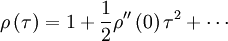
The autocorrelation can be expanded about the origin in a MacClaurin series; i.e.,
|
| (11) |

But we know the aoutocorrelation is symmetric in , hence the odd terms in must be identically to zero (i.e.,  ,
,  , etc.). Therefore the expansion of the autocorrelation near the origin reduces to:
|
| (12) |
Similary, the autocorrelation coefficient near the origin can be expanded as:
|
| (13) |
where we have used the fact that  . If we define
  we can write this compactly as:
|
| (14) |
Since  has its maximum at the origin, obviously
  must be negative.
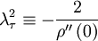
We can use the correlation and its second derivative at the origin to define a special time scale,  (called the Taylor microscale) by:
|
| (15) |
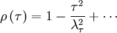
Using this in equation 14 yields the expansion for the correlation coefficient near the origin as:
|
| (16) |
Thus very near the origin the correlation coefficient (and the autocorrelation as well) simply rolls off parabolically; i.e.,
|
| (17) |
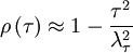
This parabolic curve is shown in Figure 3 as the osculating (or 'kissing') parabola which approaches zero exactly as the autocorrelation coefficient does. The intercept of this osculating parabola with the -axis is the Taylor microscale, .
The Taylor microscale is significant for a number of reasons. First, for many random processes (e.g., Gaussian), the Taylor microscale can be proven to be the average distance between zero-crossing of a random variable in time. This is approximately true for turbulence as well. Thus one can quickly estimate the Taylor microscale by simply observing the zero-crossings using an oscilloscope trace.
The Taylor microscale also has a special relationship to the mean square time derivative of the signal, ![\left\langle \left[ d u / d t \right]^{2} \right\rangle](/W/images/math/f/4/9/f497fde76051c4d53692efc7443bcb41.png) . This is easiest to derive if we consider two stationary random signals at two different times say
. This is easiest to derive if we consider two stationary random signals at two different times say  and
and  . The derivative of the first signal is
  and the second
  . Now lets multiply these together and rewrite them as:
|
| (18) |
where the right-hand side follows from our assumption that  is not a function of nor
  a function of .
Now if we average and interchenge the operations of differentiation and averaging we obtain:
|
| (19) |
Here comes the first trick: we simply take to be exactly but evaluated at time . So  simply becomes
  and its average is just the autocorrelation,
  . Thus we are left with:
|
| (20) |
Now we simply need to use the chain-rule. We have already defined . Let's also define  and transform the derivatives involving and to derivatives involving and
  . The result is:
|
| (21) |
So equation 20 becomes
|
| (22) |
But since  is a function only of , the derivative of it with respect to is identically zero. Thus we are left with:
|
| (23) |
And finally we need the second trick. Let's evaluate both sides at  (or
(or  ) to obtain the mean square derivative as:
|
| (24) |
But from our definition of the Taylor microscale and the facts that  and
and  , this is exactly the same as:
|
| (25) |
This amasingly simple result is very important in the study of turbulence, especially after we extend it to spatial derivatives.
Time averages of stationary processes
It is common practice in many scientific disciplines to define a time average by integrating the random variable over a fixed time interval, i.e. ,
|
| (26) |
For the stationary random processes we are considering here, we can define  to be the origin in time and simply write:
|
| (27) |
where  is the integration time.
Figure 5.4. shows a portion of a stationary random signal over which such an integration might be performed. The ime integral of  over the integral
  corresponds to the shaded area under the curve. Now since is random and since it formsthe upper boundary of the shadd area, it is clear that the time average,
  is a lot like the estimator for the mean based on a finite number of independent realization,
  we encountered earlier in section Estimation from a finite number of realizations (see Elements of statistical analysis)
It will be shown in the analysis presented below that if the signal is stationary, the time average defined by equation 27 is an unbiased estimator of the true average  . Moreover, the estimator converges to as the time becomes infinite; i.e., for stationary random processes
|
| (28) |
Thus the time and ensemble averages are equivalent in the limit as  , but only for a stationary random process.
Bias and variability of time estimators
It is easy to show that the estimator, , is unbiased by taking its ensemble average; i.e.,
|
| (29) |
Since the process has been assumed stationary,  is independent of time. It follows that:
|
| (30) |
To see whether the etimate improves as increases, the variability of must be examined, exactly as we did for earlier in section Bias and convergence of estimators (see chapter The elements of statistical analysis). To do this we need the variance of given by:
|
| (31) |
![\begin{matrix}
var \left[ U_{T} \right] & = & \left\langle \left[ U_{T} - \left\langle U_{T} \right\rangle \right]^{2} \right\rangle = \left\langle \left[ U_{T} - U \right]^{2} \right\rangle \\
& = & \frac{1}{T^{2}} \left\langle \left\{ \int^{T}_{0} \left[ u \left( t \right) - U \right] \right\}^{2} \right\rangle \\
& = & \frac{1}{T^{2}} \left\langle \int^{T}_{0} \int^{T}_{0} \left[ u \left( t \right) - U \right] \left[ u \left( t' \right) - U \right] dtdt' \right\rangle \\
& = & \frac{1}{T^{2}} \int^{T}_{0} \int^{T}_{0} \left\langle u'\left( t \right) u'\left( t' \right) \right\rangle dtdt' \\
\end{matrix}](/W/images/math/c/2/d/c2d925b6fa6871529cbd0dc983799423.png)