Introduction to turbulence/Turbulence kinetic energy

**Introduction to turbulence**
	Nature of turbulence
	Statistical analysis
	Ensemble average ; Probability ; Multivariate random var ... ; Estimation from a finite ... ; Generalization to the esti ... ;
	Reynolds averaged equation
	Turbulence kinetic energy
	Stationarity and homogeneity
	Homogeneous turbulence
	Free turbulent shear flows
	Wall bounded turbulent flows
	Study questions ... template not finished yet!

From CFD-Wiki

(Difference between revisions)

Jump to: navigation, search

Revision as of 10:46, 30 August 2007

Fluctuating kinetic energy

It is clear from the previous chapter that the straightforward application of ideas that worked well for viscous stresses do not work too well for turbulence Reynolds stresses. Moreover, even the attempt to directly derive equations for the Reynolds stresses using the Navier-Stokes equations as a starting point has left us with far more equations than unknowns. Unfortunately this means that the turbulence problem for engineers is not going to have a simple solution: we simply cannot produce a set of reasonably universal equations. Obviously we are going to have to study the turbulence fluctuations in more detail and learn how they get their energy (usually from the mean flow somehow), and what they ultimately do with it. Our hope is that by understanding more about turbulence itself, we will gain insight into how we might make closure approximations that will work, at least sometimes. Hopefully, we will also gain an understanding of when and why they will not work.

An equation for the fluctuating kinetic energy for constant density flow can be obtained directly from the Reynolds stress equation derived earlier, equation 3.35, by contracting the free indices. The result is:

$\begin{matrix} \left[ \frac{\partial}{\partial t} \left\langle u_{i} u_{i} \right\rangle + U_{j} \frac{\partial }{\partial x_{j} } \left\langle u_{i} u_{i} \right\rangle \right] \\ & = & \frac{\partial}{\partial x_{j}} \left\{ -\frac{2}{\rho} \left\langle p u_{i} \right\rangle \delta_{ij} - \left\langle q^{2} u_{j} \right\rangle + 4 \nu \left\langle s_{ij} u_{i} \right\rangle \right\} \\ & & - 2 \left\langle u_{i}u_{j} \right\rangle \frac{\partial U_{i}}{\partial x_{j}} - 4 \nu \left\langle s_{ij} \frac{\partial u_{i}}{\partial x_{j} } \right\rangle \\ \end{matrix}$

(1)

where the incompressibility condition ( $\partial u_{j} / \partial x_{j} = 0$ ) has been used to eliminate the pressure-strain rate term, and $q^{2} \equiv u_{i} u_{i}$ .

The last term can be simplified by recalling that the velocity deformation rate tensor, $\partial u_{i} / \partial x_{j}$ , can be decomposed into symmetric and anti-symmetric parts; i.e.,

$\frac{\partial u_{i}}{\partial x_{j}} = s_{ij} + \omega_{ij}$

(2)

where the symmetric part is the strain-rate tensor, $s_{ij}$ , and the anti-symmetric part is the rotation-rate tensor $\omega_{ij}$ , defined by:

$\omega_{ij} = \frac{1}{2} \left[ \frac{\partial u_{i}}{\partial x_{j}} - \frac{\partial u_{j}}{\partial x_{i}} \right]$

(3)

Since the double contraction of a symmetric tensor with an anti-symmetric tensor is identically zero, it follows immediately that:

$\begin{matrix} \left\langle s_{ij} \frac{\partial u_{i}}{\partial x_{j}} \right\rangle & = & \left\langle s_{ij} s_{ij} \right\rangle + \left\langle s_{ij} \omega_{ij} \right\rangle \\ & = & \left\langle s_{ij} s_{ij} \right\rangle \\ \end{matrix}$

(4)

Now it is customary to define a new variable k, the average fluctuating kinetic energy per unit mass, by:

$k \equiv \frac{1}{2} \left\langle u_{i}u_{i} \right\rangle = \frac{1}{2} \left\langle q^{2} \right\rangle = \frac{1}{2} \left[ \left\langle u^{2}_{1} \right\rangle + \left\langle u^{2}_{2} \right\rangle + \left\langle u^{2}_{3} \right\rangle \right]$

(5)

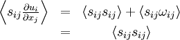
By dividing equation 1 by equation 2 and inserting this definition, the equation for the average kinetic energy per unit mass of the fluctuating motion can be re-written as:

$\begin{matrix} \left[ \frac{\partial}{\partial t} + U_{j} \frac{\partial}{\partial x_{j}} \right] k & = & \frac{\partial}{\partial x_{j}} \left\{ - \frac{1}{\rho} \left\langle pu_{i} \right\rangle \delta_{ij} - \frac{1}{2} \left\langle q^{2} u_{j} \right\rangle + 2 \nu \left\langle s_{ij}u_{i} \right\rangle \right\} \\ & & - \left\langle u_{i}u_{j} \right\rangle \frac{\partial U_{i}}{\partial x_{j} } - 2 \nu \left\langle s_{ij} s_{ij} \right\rangle \\ \end{matrix}$

(6)

The role of each of these terms will be examined in detail later. First note that an alternative form of this equation can be derived by leaving the viscous stress in terms of the strain rate. We can obtain the appropriate form of the equation for the fluctuating momentum from equation 21 in origins of turbulence by substituting the incompressible Newtonian constitutive equation into it to obtain:

$\left[ \frac{\partial }{\partial t } + U_{j} \frac{\partial }{\partial x_{j} } \right] u_{i} = - \frac{1}{\rho} \frac{\partial p}{\partial x_{i}} + \nu \frac{\partial^{2} u_{i}}{ \partial x^{2}_{j}} - \left[ u_{j} \frac{\partial U_{i}}{\partial x_{j} } \right] - \left\{ u_{j} \frac{\partial u_{i}}{ \partial x_{j}} - \left\langle u_{j} \frac{\partial u_{i}}{\partial x_{j}} \right\rangle \right\}$

(7)

If we take the scalar product of this with the fluctuating velocity itself and average, it follows (after some rearrangement) that:

$\begin{matrix} \left[ \frac{\partial}{\partial t} + U_{j} \frac{\partial}{\partial x_{j}} \right] k & = & \frac{\partial }{ \partial x_{j} } \left\{ - \frac{1}{\rho} \left\langle pu_{i} \right\rangle \delta_{ij} - \frac{1}{2} \left\langle q^{2} u_{j} \right\rangle + \nu \frac{\partial}{\partial x_{j} } k \right\} \\ & & - \left\langle u_{i} u_{j} \right\rangle \frac{\partial U_{i}}{\partial x_{j}} - \nu \left\langle \frac{\partial u_{i}}{\partial x_{j}} \frac{\partial u_{i}}{\partial x_{j}} \right\rangle\\ \end{matrix}$

(8)

Both equations 6 and 8 play an important role in the study of turbulence. The first form given by equation 6 will provide the framework for understanding the dynamics of turbulent motion. The second form, equation 8 forms the basis for most of the second-order closure attempts at turbulence modelling; e.g., the socalled k-e models ( usually referred to as the “k-epsilon models”). This because it has fewer unknowns to be modelled, although this comes at the expense of some extra assumptions about the last term. It is only the last term in equation 6 that can be identified as the true rate of dissipation of turbulence kinetic energy, unlike the last term in equation 8 which is only the dissipation when the flow is homogeneous. We will talk about homogeniety below, but suffice it to say now that it never occurs in nature. Nonetheless, many flows can be assumed to be homogeneous at the scales of turbulence which are important to this term, so-called local homogeniety.

Each term in the equation for the kinetic energy of the turbulence has a distinct role to play in the overall kinetic energy balance. Briefly these are:

Rate of change of kinetic energy per unit mass due to non-stationarity; i.e., time dependence of the mean:

$\frac{\partial k}{\partial t}$

(9)

Rate of change of kinetic energy per unit mass due to convection (or advection) by the mean flow through an inhomogenous field :

$U_{j} \frac{\partial k}{\partial x_{j}}$

(10)

Transport of kinetic energy in an inhomogeneous field due respectively to the pressure fluctuations, the turbulence itself, and the viscous stresses:

$\frac{\partial}{\partial x_{j}} \left\{-\frac{1}{\rho} \left\langle pu_{i} \right\rangle \delta_{ij} - \frac{1}{2} \left\langle q^{2} u_{j} \right\rangle + 2\nu \left\langle s_{ij}u_{i} \right\rangle \right\}$

(11)

Rate of production of turbulence kinetic energy from the mean flow(gradient):

$- \left\langle u_{i}u_{j} \right\rangle \frac{\partial U_{i}}{\partial x_{j}}$

(12)

Rate of dissipation of turbulence kinetic energy per unit mass due to viscous stresses:

$\epsilon \equiv 2\nu \left\langle s_{ij}s_{ij} \right\rangle$

(12)

These terms will be discussed in detail in the succeeding sections, and the role of each examined carefully.

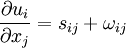
Rate of dissipation of the turbulence kinetic energy

The last term in the equation for the kinetic energy of the turbulence has been identified as the rate of dissipation of the turbulence energy per unit mass; i.e.,

$\epsilon = 2\nu \left\langle s_{ij} s_{ij} \right\rangle = \nu \left\{ \left\langle \frac{\partial u_{i} }{\partial x_{j} } \frac{\partial u_{i} }{\partial x_{j} } \right\rangle + \left\langle \frac{\partial u_{i} }{\partial x_{j} } \frac{\partial u_{j} }{\partial x_{i} } \right\rangle \right\}$

(14)

It is easy to see that $\epsilon \geq 0$ always, since it is a sum of the average of squared quantities only (i.e. $\left\langle s_{ij} s_{ij} \right\rangle \geq 0$ ). Also, since it occurs on the right hand side of the kinetic energy equation for the fluctuating motions preceded by a minus sign, it is clear that it can act only to reduce the kinetic energy of the flow. Therefore it causes a negative rate of change of kinetic energy; hence the name dissipation.

Physically, enegry is dissipated because of the work done by the fluctuating viscous stresses in resisting deformation of the fluid material by the fluctuating strain rates; i.e.

$\epsilon = \left\langle \tau^{(v)}_{ij} s_{ij} \right\rangle$

(15)

This reduces to equation 14 only for a Newtonian fluid. In non-Newtonian fluids, protions of this product may not be negative implying that it may not all represent an irrecoverable loss of fluctuating kinetic energy.

It will be shown in the following chapter on stationarity and homogenity that the dissipation of turbulence energy mostly takes place at the smallest turbulence scales, and that those scales can be characterized by so-called Kolmogorov microscale defined by:

$\eta_{K} \equiv \left(\frac{\nu^{3}}{\epsilon} \right)^{1/4}$

(16)

In atmospheric motions where the length scale for those eddies having the most turbulence energy (and responsible for the Reynolds stress) can be measured in kilometers, typical values of the Kolmogorov microscale range from 0.1 - 10 millimeters. In laboratory flows where the overall scale of the flow is greatly reduced, much smaller values of $\eta_{K}$ are not uncommon. The small size of these dissipative scales greately complicates measurement of energy balances, since the largest measuring dimension must be about equal to twice the Kolmogorov microscale. And it is the range of scales, $L / \eta$ , which makes direct numerical simulation of most interesting flows impossible, since the required number of computational cells is several orders of magnitude greater that $(L / \eta )^{3}$ . This same limitation also affects experiments as well, which must often be quite large to be useful.

One of the consequences of this great separation of scales between those containing the bulk of the turbulence energy and those dissipating it is that the dissipation rate is primarily determined by the large scales and not the small. This is because the viscous scales (which operate on a time scale of $t_{K} = ( \nu / \epsilon )^{1/2}$ ) dissipate rapidly any energy sent down to them by non-linear processes of scale to scale energy transfer. Thus the overall rate of dissipation is controlled by the rate of energy transfer from the energetic scales, primarily by the non-linear scale-to-scale transfer. This will be discussed later when we consider the energy spactrum. But for now it is important only note that a consequence of this is that the dissipation rate is given approximately as:

$\epsilon \propto \frac{u^{3}}{L}$

(17)

where $u^{2} \equiv \left\langle q^{2} \right\rangle / 3$ and $L$ is an integral length scale. It is easy to remember this relation if you note that the time scale of the energetic turbulent eddies can be estimated as $L/u$ . Thus $d3u^{2} / dt$ can estimated as $\left( 3u^{2} /2 \right) / \left( L / u \right)$ .

Sometimes it is convenient to just define the "length scale of the energy containing eddies" (or the pseudo-integral scale) as:

$l \equiv \frac{u^{3}}{\epsilon}$

(18)

Almost always $l \propto L$ , but the relation is at most only exact theoretically in the limit of infinite Reynolds number since the constant of proportionality is Reynolds number dependent. The Reynolds number dependence of the ratio $L/l$ for grid turbulence is illustrated in Figure 4.1. Many interpret this data to suggest that this ratioapproaches a constant and ignore the scatter. In fact some assume ratio to be constant and even refer to $l$ though it were the real integral scale. Others argue that the scatter is because of the differing upstream conditions and that the ratio may not be constant at all. It is really hard to tell who is right in the absence of facilities or simulations in which the Reynolds number can vary very much for fixed initial conditions. This all may leave you feeling a bit confused, but that’s the way turbulence is right now. It’s a lot easier to teach if we just tell you one view, but that’s not very good preparation for the future.

Here is what we can say for sure. Only the integral scale, $L$ , is a physical length scale, meaning that it can be directly observed in the flow by spectral or correlation measurements (as shown in the following chapters on stationarity and homogenity and homogenous turbulence). The pseudo-integral scale, $l$ , on the other hand is simply a definition; and it is only at infinite turbulence Reynolds number that it may have physical significance. But it is certainly a useful approximation at large, but finite, Reynolds numbers. We will talk about these subtle but important distinctions later when we consider homogeneous flows, but it is especially important when considering similarity theories of turbulence. For now simply file away in your memory a note of caution about using equation 17 too freely. And do not be fooled by the cute description this provides. It is just that, a description, and not really an explanation of why all this happens — sort of like the weather man describing the weather. Using equation 18, the Reynolds number dependence of the ratio of the Kolmorgorov microscale, $K$ , to the pseudo-integral scale, $l$ , can be obtained as:

$\frac{\eta_k}{l} = R_l^{-3/4}$

(19)

Figure 4.1: Ratio of physical integral length scale to pseudo-integral length scale in homogeneous turbulence as function of local Reynolds number, $R_\lambda$ .

Where the turbulence Reynolds number, $R_l$ , is defined by:

$R_l \equiv \frac{u l}{\nu} = \frac{u^4}{\nu \epsilon}$

(20)

Example: Estimate the Kolmogorov microscale for $u = 1 m/s$ and $L = 0.1 m$ for air and water.

air For air, $R_l = 1 \cdot (0.1) / 15 \cdot 10^{-6} \approx 7 \cdot 10^3$ . Therefore $l/\eta_K \approx 8 \cdot 10^2$ , so $\eta_K \approx 1.2 \cdot 10^{-4} m$ or $0.12 mm$ .

water For water, $R_l = 1 \cdot (0.1) / 10^{-6} \approx 10^5$ . Therefore $l/\eta_K \approx 5 \cdot 10^3$ , so $\eta_K \approx 2 \cdot 10^{-5} m$ or $0.02 mm$ .

Exercise: Find the dependence on $R_l$ of the time-scale ration between the Kolmorogov microtime and the time scale of the energy-containing eddies. It will also be argued later that these small dissipative scales of motion at very high Reynolds number tend to be statistically nearly isotropic; i.e., their statistical character is independent of direction. We will discuss some of the implications of isotropy and local isotropy later, but note for now that it makes possible a huge reduction in the number of unknowns, particularly those determined primarily by the dissipative scales of motion.

Thus the dissipative scales are all much smaller than those characterizing the energy of the turbulent fluctuations, and their relative size decreases with increasing Reynolds number. Note that in spite of this, the Kolmogorov scales all increase with increasing energy containing scales for fixed values of the Reynolds number. This fact is very important in designing laboratory experiments at high turbulence Reynolds number where the finite probe size limits spatial resolution. The rather imposing size of some experiments is an attempt to cope with this problem by increasing the size of the smallest scales, thus making them larger than the resolution limits of the probes being used.

Exercise: Suppose the smallest probe you can build can only resolve $0.1 mm$ . Also to do an experiment which is a reasonable model of a real engineering flow (like a hydropower plant), you need (for reason that will be clear later) a scale separation of at least $L/\eta_K = 10^4$ . If your facility has to be at least a factor of ten larger than $L$ (which you estimate as $l$ ), what is its smallest dimension?

Credits

This text was based on "Lectures in Turbulence for the 21st Century" by Professor William K. George, Professor of Turbulence, Chalmers University of Technology, Gothenburg, Sweden.

@@ Line 67: / Line 67: @@
 </td><td width="5%">(6)</td></tr></table>
-The role of each of these terms will be examined in detail later. First note that an alternative form of this equation can be derived by leaving the viscous stress in terms of the strain rate. We can obtain the appropriate form of the equation for the fluctuating momentum from equation 21 in [[Introduction to turbulence/Reynolds averaged equations#Origins of turbulence|origiins of turbulence]] by substituting the incompressible Newtonian constitutive equation into it to obtain:
+The role of each of these terms will be examined in detail later. First note that an alternative form of this equation can be derived by leaving the viscous stress in terms of the strain rate. We can obtain the appropriate form of the equation for the fluctuating momentum from equation 21 in [[Introduction to turbulence/Reynolds averaged equations#Origins of turbulence|origins of turbulence]] by substituting the incompressible Newtonian constitutive equation into it to obtain:
 <table width="70%"><tr><td>
@@ Line 155: / Line 155: @@
 This reduces to equation 14 only for a Newtonian fluid. In non-Newtonian fluids, protions of this product may not be negative implying that it may not all represent an irrecoverable loss of fluctuating kinetic energy.
-It will be shown in the following chapter on [[Introduction to turbulence/Stationarity and homogenity|Stationarity and homogenity]] that the dissipation of turbulence energy mostly takes place at the smallest turbulence scales, and that those scales can be characterized by so-called Kolmogorov microscale defined by:
+It will be shown in the following chapter on [[Introduction to turbulence/Stationarity and homogenity|stationarity and homogenity]] that the dissipation of turbulence energy mostly takes place at the smallest turbulence scales, and that those scales can be characterized by so-called Kolmogorov microscale defined by:
 <table width="70%"><tr><td>
@@ Line 183: / Line 183: @@
 </td><td width="5%">(18)</td></tr></table>
-Almost always <math> l \propto L </math>, but the relation is at most only exact theoretically in the limit of infinite Reynolds number since the constant of proportionality is Reynolds number dependent. The Reynolds number dependence of the ratio <math> L/l </math> for grid turbulence is illustrated in <font color=orange>Figure 4.1</font>. Many interpret this data to suggest that this ratioapproaches a constant and ignore the scatter. In fact some assume ratio to be constant and even refer to <math> l </math> though it were the real integral scale. Others
+Almost always <math> l \propto L </math>, but the relation is at most only exact theoretically in the limit of infinite Reynolds number since the constant of proportionality is Reynolds number dependent. The Reynolds number dependence of the ratio <math> L/l </math> for grid turbulence is illustrated in <font color=orange>Figure 4.1</font>. Many interpret this data to suggest that this ratioapproaches a constant and ignore the scatter. In fact some assume ratio to be constant and even refer to <math> l </math> though it were the real integral scale. Others argue that the scatter is because of the differing upstream conditions and that the ratio may not be constant at all. It is really hard to tell who is right in the absence of facilities or simulations in which the Reynolds number can vary very much for fixed initial conditions. This all may leave you feeling a bit confused, but that’s the way turbulence is right now. It’s a lot easier to teach if we just tell you one view, but that’s not very good preparation for the future.
-argue that the scatter is because of the differing upstream conditions and that the ratio may not be constant at all. It is really hard to tell who is right in the absence of facilities or simulations in which the Reynolds number can vary very much for fixed initial conditions. This all may leave you feeling a bit confused, but that’s the way turbulence is right now. It’s a lot easier to teach if we just tell you one view, but that’s not very good preparation for the future.
+Here is what we can say for sure. Only the integral scale, <math>L</math>, is a physical length scale, meaning that it can be directly observed in the flow by spectral or correlation measurements (as shown in the following chapters on [[Introduction to turbulence/Stationarity and homogenity|stationarity and homogenity]] and [[Introduction to turbulence/Homogenous turbulence|homogenous turbulence]]). The pseudo-integral scale, <math>l</math>, on the other hand is simply a definition; and it is only at infinite turbulence Reynolds number that it may have physical significance. But it is certainly a useful
+approximation at large, but finite, Reynolds numbers. We will talk about these subtle but important distinctions later when we consider homogeneous flows, but it is especially important when considering similarity theories of turbulence. For
+now simply file away in your memory a note of caution about using equation 17 too freely. And do not be fooled by the cute description this provides. It is just that, a description, and not really an explanation of why all this happens — sort
+of like the weather man describing the weather. Using equation 18, the Reynolds number dependence of the ratio of the
+Kolmorgorov microscale, <math>K</math>, to the pseudo-integral scale, <math>l</math>, can be obtained as:
+<table width="70%"><tr><td>
+:<math>
+\frac{\eta_k}{l} = R_l^{-3/4}
+</math>
+</td><td width="5%">(19)</td></tr></table>
+Figure 4.1: Ratio of physical integral length scale to pseudo-integral length scale in homogeneous turbulence as function of local Reynolds number, <math>R_\lambda</math>.
+Where the turbulence Reynolds number, <math>R_l</math>, is defined by:
+<table width="70%"><tr><td>
+:<math>
+R_l \equiv \frac{u l}{\nu} = \frac{u^4}{\nu \epsilon}
+</math>
+</td><td width="5%">(20)</td></tr></table>
+'''Example:''' Estimate the Kolmogorov microscale for <math>u = 1 m/s</math> and <math>L = 0.1 m</math> for air and water.
+:'''air''' For air, <math>R_l = 1 \cdot (0.1) / 15 \cdot 10^{-6} \approx 7 \cdot 10^3 </math>. Therefore <math>l/\eta_K \approx 8 \cdot 10^2</math>, so <math>\eta_K \approx 1.2 \cdot 10^{-4} m</math> or <math>0.12 mm</math>.
+:'''water''' For water, <math>R_l = 1 \cdot (0.1) / 10^{-6} \approx 10^5 </math>. Therefore <math>l/\eta_K \approx 5 \cdot 10^3</math>, so <math>\eta_K \approx 2 \cdot 10^{-5} m</math> or <math>0.02 mm</math>.
+'''Exercise:''' Find the dependence on <math>R_l</math> of the time-scale ration between the Kolmorogov microtime and the time scale of the energy-containing eddies. It will also be argued later that these small dissipative scales of motion at very
+high Reynolds number tend to be statistically nearly isotropic; i.e., their statistical character is independent of direction. We will discuss some of the implications of isotropy and local isotropy later, but note for now that it makes possible a huge
+reduction in the number of unknowns, particularly those determined primarily by the dissipative scales of motion.
+Thus the dissipative scales are all much smaller than those characterizing the energy of the turbulent fluctuations, and their relative size decreases with increasing Reynolds number. Note that in spite of this, the Kolmogorov scales all increase
+with increasing energy containing scales for fixed values of the Reynolds number. This fact is very important in designing laboratory experiments at high turbulence Reynolds number where the finite probe size limits spatial resolution. The
+rather imposing size of some experiments is an attempt to cope with this problem by increasing the size of the smallest scales, thus making them larger than the resolution limits of the probes being used.
+'''Exercise:''' Suppose the smallest probe you can build can only resolve <math>0.1 mm</math>. Also to do an experiment which is a reasonable model of a real engineering flow (like a hydropower plant), you need (for reason that will be clear later) a scale separation of at least <math>L/\eta_K = 10^4</math>. If your facility has to be at least a factor of ten larger than <math>L</math> (which you estimate as <math>l</math>), what is its smallest dimension?
 {{Turbulence credit wkgeorge}}
 {{Chapter navigation|Reynolds averaged equations|Stationarity and homogenity}}

Introduction to turbulence/Turbulence kinetic energy

From CFD-Wiki

Revision as of 10:46, 30 August 2007

Fluctuating kinetic energy

Rate of dissipation of the turbulence kinetic energy

Credits

Views

My wiki

wiki navigation

wiki search

wiki toolbox