Kato-Launder modification
From CFD-Wiki
| Line 68: | Line 68: | ||
</math> | </math> | ||
| - | == | + | ==Production term modification== |
| - | The proposal by Kato and Launder is to replace one of the strain-rates, <math>S</math>, in the vorticity, <math>\Omega</math> | + | The proposal by Kato and Launder is to replace one of the strain-rates, <math>S</math>, in the turbulent production term, <math>P</math>, above with the vorticity, <math>\Omega</math>. |
| - | + | The Kato-Launder modified production term then becomes: | |
:<math> | :<math> | ||
| Line 89: | Line 89: | ||
S \equiv \sqrt{\frac{1}{2} \left( \frac{\partial u_i}{\partial x_j} - \frac{\partial u_j}{\partial x_i} \right)^2 } | S \equiv \sqrt{\frac{1}{2} \left( \frac{\partial u_i}{\partial x_j} - \frac{\partial u_j}{\partial x_i} \right)^2 } | ||
</math> | </math> | ||
| + | |||
| + | In pure shear-flows like boundary-layers and wakes the Kato-Launder modified production term will give exactly the same result as the unmodified production term because in these flows the strain-rate is equal to the vorticity. | ||
==References== | ==References== | ||
{{reference-paper|author=Kato, M. and Launder, B. E.|year=1993|title=The Modeling of Turbulent Flow Around Stationary and Vibrating Square Cylinders|rest=Proc. 9th Symposium on Turbulent Shear Flows, Kyoto, August 1993, pp. 10.4.1-10.4.6}} | {{reference-paper|author=Kato, M. and Launder, B. E.|year=1993|title=The Modeling of Turbulent Flow Around Stationary and Vibrating Square Cylinders|rest=Proc. 9th Symposium on Turbulent Shear Flows, Kyoto, August 1993, pp. 10.4.1-10.4.6}} | ||
Revision as of 15:45, 8 December 2005
The Kato-Launder modification is an ad-hoc modification of the turbulent production term in the k equation. The main purpose of the modification is to reduce the tendency that two-equation models have to over-predict the turbulent production in regions with large normal strain, i.e. regions with strong acceleration or decelleration.
Basic equations
The transport equation for the turbulent energy,  , used in most two-equation models can be written as:
![\frac{\partial}{\partial t} \left( \rho k \right) +
\frac{\partial}{\partial x_j}
\left[
\rho k u_j - \left( \mu + \frac{\mu_t}{\sigma_k} \right)
\frac{\partial k}{\partial x_j}
\right]
=
P - \rho \epsilon - \rho D](/W/images/math/8/d/7/8d787db6600e44ff6855992620431595.png)
Where  is the turbulent production normally given by:
 is the turbulent shear stress tensor given by the Boussinesq assumption:
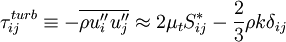
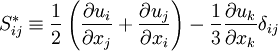
Where  is the eddy-viscosity given by the turbluence model and
  is the trace-less viscous strain-rate defined by:
In incompressible flows, where  , the production term can be rewritten as:
![\begin{matrix}
P & = & \tau_{ij}^{turb} \frac{\partial u_i}{\partial x_j} \\
\ & = & \left[ 2 \mu_t S_{ij}^* - \frac{2}{3} \rho k \delta_{ij} \right] \frac{\partial u_i}{\partial x_j} \\
\ & = & \left[ 2 \mu_t \left( \frac{1}{2} \left(\frac{\partial u_i}{\partial x_j} +
\frac{\partial u_j}{\partial x_i} \right) - \frac{1}{3} \frac{\partial u_k}{\partial x_k} \delta_{ij} \right)
- \frac{2}{3} \rho k \delta_{ij}
\right] \frac{\partial u_i}{\partial x_j} \\
\ & \approx & \mu_t \left(\frac{\partial u_i}{\partial x_j} +
\frac{\partial u_j}{\partial x_i} \right) \frac{\partial u_i}{\partial x_j} \\
\ & = & \mu_t \frac{1}{2} \left(\frac{\partial u_i}{\partial x_j} + \frac{\partial u_j}{\partial x_i} \right)
\left(\frac{\partial u_i}{\partial x_j} + \frac{\partial u_j}{\partial x_i} \right) \\
\end{matrix}](/W/images/math/c/2/e/c2edca17cad100ee94b91f1ebc9516c5.png)
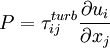
Hence

Where

Production term modification
The proposal by Kato and Launder is to replace one of the strain-rates,  , in the turbulent production term, , above with the vorticity,
  .
.
The Kato-Launder modified production term then becomes:
Where
and
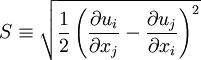
In pure shear-flows like boundary-layers and wakes the Kato-Launder modified production term will give exactly the same result as the unmodified production term because in these flows the strain-rate is equal to the vorticity.
References
Kato, M. and Launder, B. E. (1993), "The Modeling of Turbulent Flow Around Stationary and Vibrating Square Cylinders", Proc. 9th Symposium on Turbulent Shear Flows, Kyoto, August 1993, pp. 10.4.1-10.4.6.