Linear wave propagation

From CFD-Wiki

Revision as of 06:25, 14 January 2006 (view source) Harish gopalan (Talk | contribs) ← Older edit		Revision as of 07:14, 14 January 2006 (view source) Harish gopalan (Talk | contribs) Newer edit →
Line 3:		Line 3:
	</math>		</math>
	== Domain ==		== Domain ==
-	x=[0,1]	+	:<math> x=[-10,10] </math>
	== Initial Condition ==		== Initial Condition ==
-	:<math> u(x,0)=e^{-360*{(x-0.25)}^2}</math>	+	:<math> u(x,0)=exp[-ln(2){(\frac{x-x_c}{r})}^2]</math>
	== Boundary condition ==		== Boundary condition ==
-	u[0]=0,u[imax]=u[imax-1](x[imax]=1.0)	+	:<math>u(-10)=0</math>
	== Exact solution ==		== Exact solution ==
-	:<math> u(x,t)=e^{-360*{((x-c*t)-0.25)}^2}</math>	+	:<math> u(x,0)=exp[-ln(2){(\frac{x-x_c-ct}{r})}^2]</math>
	== Numerical method ==		== Numerical method ==
-	c=1,t=0.25	+	:<math>c=1,dx=1/6,dt=0.5dx,t=7.5</math>
		+	:<math> \mbox{Long wave  :}\frac{r}{dx}=20</math>
		+	:<math> \mbox{Medium wave: }\frac{r}{dx}=6</math>
		+	:<math> \mbox{Short wave : } \frac{r}{dx}=3</math>
		+	=== Space ===
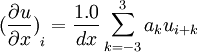
		+	==== Explicit Scheme (DRP)====
		+	:<math> {(\frac{\partial u}{\partial x})}_i=\frac{1.0}{dx}\sum_{k=-3}^3 a_k u_{i+k} </math>
		+	The coefficients can be found in Tam(1992).At the right boundaries use fourth order central difference and fourth backward difference.At left boundaries use second order central difference for i=2 and fourth order central difference for i=3.The Dispersion relation preserving (DRP) finite volume scheme can be found in Popescu (2005).
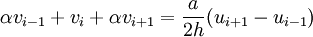
		+	====Implicit Scheme(Compact)====
		+	:Domain: <math>\alpha v_{i-1} + v_i + \alpha v_{i+1}=\frac{a}{2h}(u_{i+1}-u_{i-1}) </math>
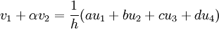
		+	:Boundaries: <math> v_1+\alpha v_2=\frac{1}{h}(au_1+bu_2+cu_3+du_4) </math>
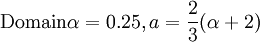
		+	where v refers to the first derivative.For a general treatment of compact scheme refer to Lele (1992).In this test case the following values are used
		+	:<math> \mbox{Domain} \alpha=0.25 , a=\frac{2}{3}(\alpha+2) </math>
		+	:<math> \mbox{Boundary} \alpha=2 ,a=-(\frac{11+2\alpha}{6}),b=\frac{6-\alpha}{2},c=\frac{2\alpha-3}{2},d=\frac{2-\alpha}{6} </math>
		+
	== Results ==		== Results ==
		+
	[[Image:Initial_condition.png|450px]]		[[Image:Initial_condition.png|450px]]
	[[Image:Result_wave.png|450px]]		[[Image:Result_wave.png|450px]]
	== Reference ==		== Reference ==

---

Revision as of 07:14, 14 January 2006

Contents 1 Problem definition 2 Domain 3 Initial Condition 4 Boundary condition 5 Exact solution 6 Numerical method 6.1 Space 6.1.1 Explicit Scheme (DRP) 6.1.2 Implicit Scheme(Compact) 7 Results 8 Reference

Problem definition

Domain

Initial Condition

Boundary condition

Exact solution

Numerical method

Space

Explicit Scheme (DRP)

The coefficients can be found in Tam(1992).At the right boundaries use fourth order central difference and fourth backward difference.At left boundaries use second order central difference for i=2 and fourth order central difference for i=3.The Dispersion relation preserving (DRP) finite volume scheme can be found in Popescu (2005).

Implicit Scheme(Compact)

Domain:

Boundaries:

where v refers to the first derivative.For a general treatment of compact scheme refer to Lele (1992).In this test case the following values are used

Results

Reference