Probability density function
From CFD-Wiki
(Corrected the variance equation.) |
|||
| (8 intermediate revisions not shown) | |||
| Line 6: | Line 6: | ||
:<math> | :<math> | ||
| - | F_\phi(\Phi) = p(phi < \Phi) | + | F_\phi(\Phi) = p(\phi < \Phi) |
</math> | </math> | ||
| Line 13: | Line 13: | ||
:<math> | :<math> | ||
| - | p(\Phi_1 <phi < \Phi_2) = F_\phi(\Phi_2)-F_\phi(\Phi_1) | + | p(\Phi_1 <\phi < \Phi_2) = F_\phi(\Phi_2)-F_\phi(\Phi_1) |
</math> | </math> | ||
| Line 26: | Line 26: | ||
\int P(\Phi) d \Phi = 1 | \int P(\Phi) d \Phi = 1 | ||
</math> | </math> | ||
| - | Integrating over all the possible values of <math> \phi </math>. | + | Integrating over all the possible values of <math> \phi </math>, |
| + | <math> \Phi </math> is the sample space of the scalar variable <math> \phi </math>. | ||
The PDF of any stochastic variable depends "a-priori" on space and time. | The PDF of any stochastic variable depends "a-priori" on space and time. | ||
:<math> P(\Phi;x,t) </math> | :<math> P(\Phi;x,t) </math> | ||
| + | for clarity of notation, the space and time dependence is dropped. | ||
| + | <math> P(\Phi) \equiv P(\Phi;x,t) </math> | ||
| + | |||
| + | |||
| + | From the PDF of a variable, one can define its <math> n </math>th moment as | ||
| + | |||
| + | :<math> | ||
| + | \overline{\phi}^n = \int \phi^n P(\Phi) d \Phi | ||
| + | </math> | ||
| + | |||
| + | the <math> n = 1 </math> case is called the "mean". | ||
| + | |||
| + | :<math> | ||
| + | \overline{\phi} = \int \phi P(\Phi) d \Phi | ||
| + | </math> | ||
| + | |||
| + | Similarly the mean of a function can be obtained as | ||
| + | |||
| + | :<math> | ||
| + | \overline{f} = \int f(\phi) P(\Phi) d \Phi | ||
| + | </math> | ||
| + | |||
| + | Where the second central moment is called the "variance" | ||
| + | |||
| + | :<math> | ||
| + | \overline{u'^2} = \int (\phi-\overline{\phi})^2 P(\Phi) d \Phi | ||
| + | </math> | ||
| + | |||
| + | For two variables (or more) a joint-PDF of <math> \phi </math> and <math> \psi </math> is defined | ||
| + | :<math> P(\Phi,\Psi;x,t) \equiv P (\Phi,\Psi) </math> | ||
| + | |||
| + | where <math> \Phi \mbox{ and } \Psi </math> form the phase-space for | ||
| + | <math> \phi \mbox{ and } \psi </math>. | ||
| + | The marginal PDF's are obtained by integration over the sample space of one variable. | ||
| + | :<math> | ||
| + | P(\Phi) = \int P(\Phi,\Psi) d\Psi | ||
| + | </math> | ||
| + | |||
| + | For two variables the correlation is given by | ||
| + | |||
| + | :<math> | ||
| + | \overline{\phi' \psi'} = \int (\phi-\overline{\phi}) (\psi-\overline{\psi}) P(\Phi,\Psi) d \Phi d\Psi | ||
| + | </math> | ||
| + | |||
| + | This term often appears in turbulent flows the averaged Navier-Stokes (with <math> u, v </math>) and is unclosed. | ||
| + | |||
| + | Using Bayes' theorem a joint-pdf can be expressed as | ||
| + | :<math> | ||
| + | P(\Phi,\Psi) = P(\Phi|\Psi) P(\Psi) | ||
| + | </math> | ||
| + | where <math> P(\Phi|\Psi) </math> is the conditional PDF. | ||
| + | |||
| + | The conditional average of a scalar can be expressed as a function of the | ||
| + | conditional PDF | ||
| + | :<math> | ||
| + | <\phi | \Psi > = \int \phi P(\Phi|\Psi) d \Phi | ||
| + | </math> | ||
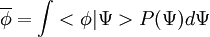
| + | and the mean value of a scalar can be expressed | ||
| + | |||
| + | :<math> | ||
| + | \overline{\phi} = \int <\phi | \Psi > P(\Psi) d \Psi | ||
| + | </math> | ||
| + | only if <math> \phi </math> and <math> \psi </math> are correlated. | ||
| + | |||
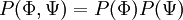
| + | If two variables are uncorrelated then they are statistically independent and their joint PDF can be expressed as a product of their marginal PDFs. | ||
| + | :<math> | ||
| + | P(\Phi,\Psi)= P(\Phi) P(\Psi) | ||
| + | </math> | ||
| + | |||
| + | |||
| + | Finally a joint PDF of <math> N </math> scalars <math> (\phi_1,\phi_2, ...,\phi_N) </math> | ||
| + | is defined as | ||
| + | :<math> | ||
| + | P(\underline{\psi}; x,t) \equiv P(\underline{\psi}) | ||
| + | </math> | ||
| + | where <math> \underline{\psi} = (\psi_1,\psi_2, ...,\psi_N) </math> is the sample space of the array | ||
| + | <math> \underline{\phi} </math>. | ||
Latest revision as of 16:03, 20 May 2011
Stochastic methods use distribution functions to decribe the fluctuacting scalars in a turbulent field.
The distribution function  of a scalar
  is the probability
 of finding a value of
The probability of finding in a range  is
is

The probability density function (PDF) is
where  is the probability of being in the range
  . It follows that
Integrating over all the possible values of ,
 is the sample space of the scalar variable .
The PDF of any stochastic variable depends "a-priori" on space and time.
is the sample space of the scalar variable .
The PDF of any stochastic variable depends "a-priori" on space and time.

for clarity of notation, the space and time dependence is dropped.
From the PDF of a variable, one can define its  th moment as
the  case is called the "mean".
Similarly the mean of a function can be obtained as
Where the second central moment is called the "variance"
For two variables (or more) a joint-PDF of and  is defined
where  form the phase-space for
 .
The marginal PDF's are obtained by integration over the sample space of one variable.
.
The marginal PDF's are obtained by integration over the sample space of one variable.
For two variables the correlation is given by
This term often appears in turbulent flows the averaged Navier-Stokes (with  ) and is unclosed.
Using Bayes' theorem a joint-pdf can be expressed as

where  is the conditional PDF.
The conditional average of a scalar can be expressed as a function of the conditional PDF
and the mean value of a scalar can be expressed
only if and are correlated.
If two variables are uncorrelated then they are statistically independent and their joint PDF can be expressed as a product of their marginal PDFs.
Finally a joint PDF of  scalars
  is defined as
where  is the sample space of the array
 .
.