Source term linearization
From CFD-Wiki
Revision as of 05:44, 7 December 2005
Introduction
In seeking the solution of the general transport equation for a scalar  , the main objective is to correctly handle the non-linearities by transforming them into linear form and then iteratively account for the non-linearity. The source term plays a central role in this respect when it is non-linear. For example, in radiation heat transfer, the source term in energy equation is expressed as fourth powers in the temperature.
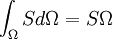
When the source is constant and independent of the conserved scalar, the finite volume method assumes that the value of S prevails of the control volume and thus can be easily integrated. For a given control volume P, we obtain
Picard's Method
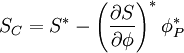
Picard's method is the most popular method used in conjunction with the finite volume method. For a given control volume P, we start by writing the source term as
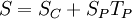
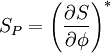
where  denotes the constant part of S and
  denotes the coefficient of
  (not the value of S at P). This allows ups to account for
  in the coefficients for .
Let  denote the value of at the current itertaion. We now write a Taylor series expansion of S about as
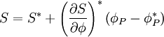
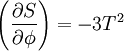
therefore
where  is the gradient of S evaluated at .
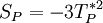
As an illustrative example, consider  . Following Picard's method, we have