|
|
|
[Sponsors] | ||||
Hypersonic simulation on nozzle convergent-divergent |
 |
|
|
LinkBack | Thread Tools | Search this Thread | Display Modes |
 October 17, 2015, 12:56
|
|
#1 |
|
New Member
Antonio Lattanziu
Join Date: Jul 2013
Posts: 6
Rep Power: 12  |
Hi guys, I created a mesh within pointwise and am trying to do the simulations on a convergent-divergent nozzle considering the model of dissociation N2. When I do the simulation I get the following error:
----------------------------- Begin Solver ----------------------------- Segmentation fault (core dumped) The boundary condition it is: i=1: Subsonic inlet, pt = 100 atm, Tt = 5600 K (stagnation conditions) i=IMAX: Free stream j=1: Symmetry conditions j=JMAX: Inviscid wall. The configuration file it is: COMPRESSIBLE FREE-STREAM DEFINITION Mach number (non-dimensional, based on the free-stream values) MACH_NUMBER= 23.9 % % Angle of attack (degrees, only for compressible flows) AoA= 0.0 % % Side-slip angle (degrees, only for compressible flows) SIDESLIP_ANGLE= 0.0 % % Free-stream pressure (101325.0 N/m^2 by default) FREESTREAM_PRESSURE= 19.7594 % % Free-stream temperature (288.15 K by default) FREESTREAM_TEMPERATURE= 254.0 % % Free-stream vibrational-electronic temperature (288.15 K by default) FREESTREAM_TEMPERATURE_VE= 254.0 % % Reynolds number (non-dimensional, based on the free-stream values) REYNOLDS_NUMBER= 19500 % % Reynolds length (1 m by default) REYNOLDS_LENGTH= 1.0 % ---------------------- REFERENCE VALUE DEFINITION ---------------------------% % % Reference origin for moment computation REF_ORIGIN_MOMENT_X = 0.00 REF_ORIGIN_MOMENT_Y = 0.00 REF_ORIGIN_MOMENT_Z = 0.00 % % Reference length for pitching, rolling, and yawing non-dimensional moment REF_LENGTH_MOMENT= 1.0 % % Reference area for force coefficients (0 implies automatic calculation) REF_AREA= 1.0 % -------------------- BOUNDARY CONDITION DEFINITION --------------------------% % % Euler wall boundary marker(s) (NONE = no marker) MARKER_EULER= ( Inviscid_wall ) MARKER_INLET= ( Inlet, 300, 19956.1, 1.0, 0.0, 0.0 ) % % Far-field boundary marker(s) (NONE = no marker) MARKER_FAR= ( Inflow, Outflow, Top ) % % Symmetry boundary marker(s) (NONE = no marker) MARKER_SYM= ( Symmetry ) MARKER_OUTLET= ( Outlet, 101300 ) % ------------------------ SURFACES IDENTIFICATION ----------------------------% % % Marker(s) of the surface in the surface flow solution file MARKER_PLOTTING = ( Wall ) % % Marker(s) of the surface where the non-dimensional coefficients are evaluated. MARKER_MONITORING = ( Wall ) % % Marker(s) of the surface where obj. func. (design problem) will be evaluated MARKER_DESIGNING = ( Wall ) % ------------- COMMON PARAMETERS DEFINING THE NUMERICAL METHOD ---------------% % % Numerical method for spatial gradients (GREEN_GAUSS, WEIGHTED_LEAST_SQUARES) NUM_METHOD_GRAD= WEIGHTED_LEAST_SQUARES % % Courant-Friedrichs-Lewy condition of the finest grid CFL_NUMBER= 0.5 % % Adaptive CFL number (NO, YES) CFL_ADAPT= NO % % Parameters of the adaptive CFL number (factor down, factor up, CFL min value, % CFL max value ) CFL_ADAPT_PARAM= ( 1.5, 0.5, 1.0, 100.0 ) % % Runge-Kutta alpha coefficients RK_ALPHA_COEFF= ( 0.66667, 0.66667, 1.000000 ) % % Number of total iterations EXT_ITER= 3000 % ------------------------ LINEAR SOLVER DEFINITION ---------------------------% % % Linear solver for the implicit (or discrete adjoint) formulation (LU_SGS, % SYM_GAUSS_SEIDEL, BCGSTAB, GMRES) LINEAR_SOLVER= FGMRES % % Linear solver preconditioner LINEAR_SOLVER_PREC= LU_SGS % % Min error of the linear solver for the implicit formulation LINEAR_SOLVER_ERROR= 1E-8 % % Max number of iterations of the linear solver for the implicit formulation LINEAR_SOLVER_ITER= 10 % -------------------------- MULTIGRID PARAMETERS -----------------------------% % % Multi-grid Levels (0 = no multi-grid) MGLEVEL= 0 % % Multi-grid cycle (V_CYCLE, W_CYCLE, FULLMG_CYCLE) MGCYCLE= V_CYCLE % % Multi-grid pre-smoothing level MG_PRE_SMOOTH= ( 1, 2, 3, 3 ) % % Multi-grid post-smoothing level MG_POST_SMOOTH= ( 0, 0, 0, 0 ) % % Jacobi implicit smoothing of the correction MG_CORRECTION_SMOOTH= ( 0, 0, 0, 0 ) % % Damping factor for the residual restriction MG_DAMP_RESTRICTION= 0.85 % % Damping factor for the correction prolongation MG_DAMP_PROLONGATION= 0.85 % -------------------- FLOW NUMERICAL METHOD DEFINITION -----------------------% % % Convective numerical method (JST, LAX-FRIEDRICH, CUSP, ROE, AUSM, HLLC, % TURKEL_PREC, MSW) CONV_NUM_METHOD_FLOW= AUSM % % Spatial numerical order integration (1ST_ORDER, 2ND_ORDER, 2ND_ORDER_LIMITER) % SPATIAL_ORDER_FLOW= 2ND_ORDER % % Slope limiter (VENKATAKRISHNAN, MINMOD) SLOPE_LIMITER_FLOW= VENKATAKRISHNAN % % Coefficient for the limiter LIMITER_COEFF= 0.3 % % 1st, 2nd and 4th order artificial dissipation coefficients AD_COEFF_FLOW= ( 0.15, 0.5, 0.02 ) % % Time discretization (RUNGE-KUTTA_EXPLICIT, EULER_IMPLICIT, EULER_EXPLICIT) TIME_DISCRE_FLOW= EULER_IMPLICIT % -------------------- TNE2 NUMERICAL METHOD DEFINITION -----------------------% % % Convective numerical method (ROE, AUSM, HLLC) CONV_NUM_METHOD_TNE2= AUSM % % Spatial numerical order integration (1ST_ORDER, 2ND_ORDER, 2ND_ORDER_LIMITER) % SPATIAL_ORDER_TNE2= 1ST_ORDER % % Slope limiter (VENKATAKRISHNAN) SLOPE_LIMITER_TNE2= VENKATAKRISHNAN % % Time discretization (RUNGE-KUTTA_EXPLICIT, EULER_IMPLICIT, EULER_EXPLICIT) TIME_DISCRE_TNE2= EULER_IMPLICIT % ----------------------- GEOMETRY EVALUATION PARAMETERS ----------------------% % % Geometrical evaluation mode (ANALYSIS, GRADIENT) GEO_MODE= GRADIENT % --------------------------- CONVERGENCE PARAMETERS --------------------------% % % Convergence criteria (CAUCHY, RESIDUAL) % CONV_CRITERIA= RESIDUAL % % Residual reduction (order of magnitude with respect to the initial value) RESIDUAL_REDUCTION= 5 % % Min value of the residual (log10 of the residual) RESIDUAL_MINVAL= -8 % % Start convergence criteria at iteration number STARTCONV_ITER= 10 % % Number of elements to apply the criteria CAUCHY_ELEMS= 100 % % Epsilon to control the series convergence CAUCHY_EPS= 1E-10 % % Function to apply the criteria (LIFT, DRAG, NEARFIELD_PRESS, SENS_GEOMETRY, % SENS_MACH, DELTA_LIFT, DELTA_DRAG) CAUCHY_FUNC_FLOW= DRAG CAUCHY_FUNC_ADJFLOW= SENS_GEOMETRY the mesh it is: 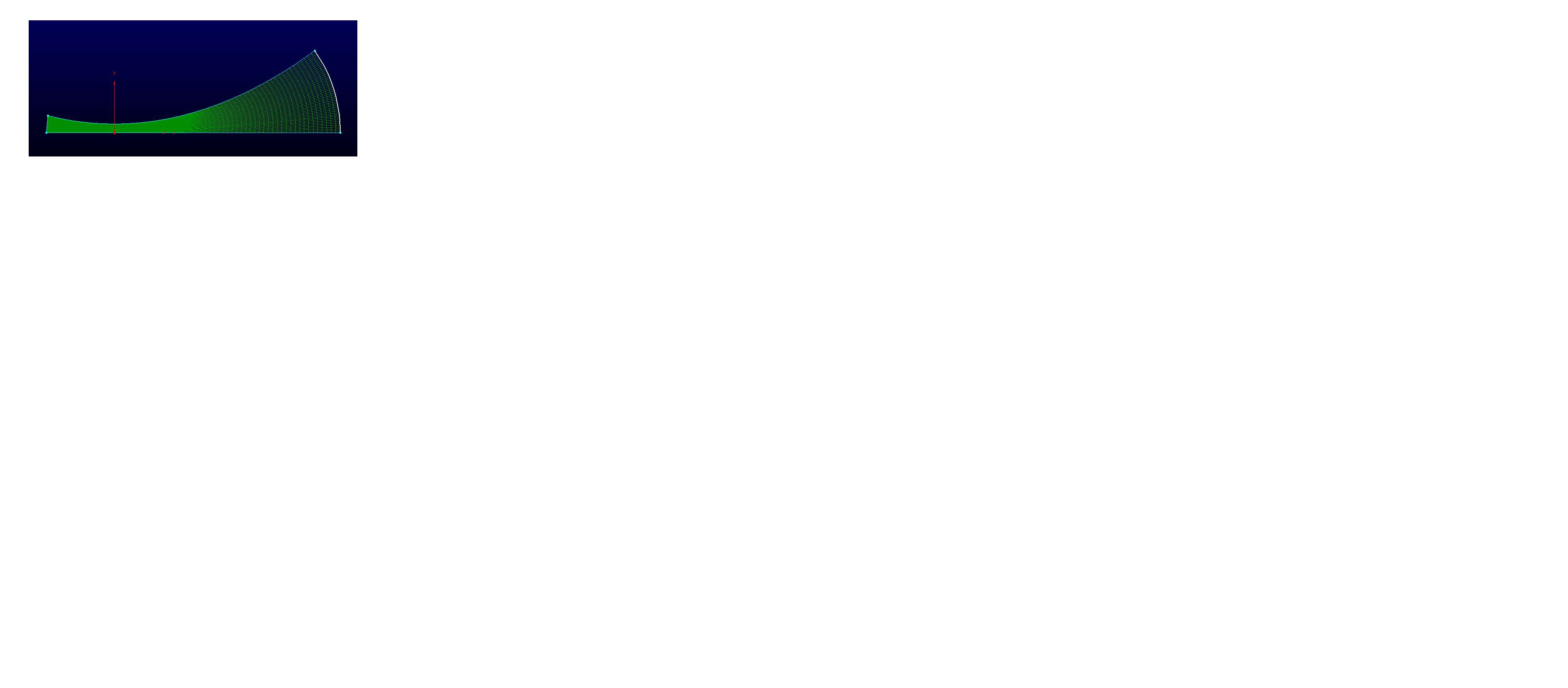 I would be grateful for any help you could provide. Thanks. |
|

|

|
|
|
October 22, 2015, 11:24
|
|
#2 |
|
Super Moderator
Tim Albring
Join Date: Sep 2015
Posts: 195
Rep Power: 10 |
Hi tonino,
the most important part is missing: what about the math problem options (probably just a copy & paste thing). Then you reference some boundary markers that are not existent in your mesh I guess (Wall, Inflow, Outflow, Top). So remove the option MARKER_FAR and set MARKER_{PLOTTING, MONITORING, DESIGNING) to ( Inviscid_Wall ). Maybe this already helps. |
|
|
|
|
|
|
November 19, 2016, 06:26
|
|
#3 |
|
New Member
Amitava Mandal
Join Date: Oct 2016
Posts: 6
Rep Power: 9 |
In regard to the above mentioned problem, I have the following queries.
1. Reynold no, corresponding to which condition? 2. Which is the ideal boundary condition for this case i.e. supersonic or pressure boundary? Regards Amitava Mandal |
|
|
|
|
|
|
|
|
 Similar Threads
|
||||
| Thread | Thread Starter | Forum | Replies | Last Post |
| having trouble modelling basic convergent water nozzle flow | derhamp | STAR-CCM+ | 1 | January 14, 2016 16:37 |
| Residuals high for 2D Convergent divergent nozzle simulation | jphoenix | FLUENT | 0 | November 11, 2014 08:12 |
| Need help with a rocket nozzle simulation | badboyz31 | CFX | 14 | September 22, 2014 00:06 |
| Jet exhaust from the nozzle simulation | Krafta | OpenFOAM | 0 | September 2, 2014 12:30 |
| mass flow rate issue in supersonic nozzle simulation | xkang | FLUENT | 0 | July 31, 2014 16:06 |
 Linear Mode


