Introduction to turbulence/Turbulence kinetic energy
From CFD-Wiki
| Nature of turbulence |
| Statistical analysis |
| Reynolds averaged equation |
| Turbulence kinetic energy |
| Stationarity and homogeneity |
| Homogeneous turbulence |
| Free turbulent shear flows |
| Wall bounded turbulent flows |
| Study questions
... template not finished yet! |
Contents |
Fluctuating kinetic energy
It is clear from the previous chapter that the straightforward application of ideas that worked well for viscous stresses do not work too well for turbulence Reynolds stresses. Moreover, even the attempt to directly derive equations for the Reynolds stresses using the Navier-Stokes equations as a starting point has left us with far more equations than unknowns. Unfortunately this means that the turbulence problem for engineers is not going to have a simple solution: we simply cannot produce a set of reasonably universal equations. Obviously we are going to have to study the turbulence fluctuations in more detail and learn how they get their energy (usually from the mean flow somehow), and what they ultimately do with it. Our hope is that by understanding more about turbulence itself, we will gain insight into how we might make closure approximations that will work, at least sometimes. Hopefully, we will also gain an understanding of when and why they will not work.
An equation for the fluctuating kinetic energy for constant density flow can be obtained directly from the Reynolds stress equation derived earlier (see equation 35 in the chapter on Reynolds averaged equations) by contracting the free indices. The result is:
|
| (1) |
![\begin{matrix}
\left[ \frac{\partial}{\partial t} \left\langle u_{i} u_{i} \right\rangle + U_{j} \frac{\partial }{\partial x_{j} } \left\langle u_{i} u_{i} \right\rangle \right] \\
& = & \frac{\partial}{\partial x_{j}} \left\{ -\frac{2}{\rho} \left\langle p u_{i} \right\rangle \delta_{ij} - \left\langle q^{2} u_{j} \right\rangle + 4 \nu \left\langle s_{ij} u_{i} \right\rangle \right\} \\
& & - 2 \left\langle u_{i}u_{j} \right\rangle \frac{\partial U_{i}}{\partial x_{j}} - 4 \nu \left\langle s_{ij} \frac{\partial u_{i}}{\partial x_{j} } \right\rangle \\
\end{matrix}](/W/images/math/c/d/d/cdd713e7c866ab3a41c1db5df222a7b2.png)
where the incompressibility condition (  ) has been used to eliminate the pressure-strain rate term, and
  .
.
The last term can be simplified by recalling that the velocity deformation rate tensor,  , can be decomposed into symmetric and anti-symmetric parts; i.e.,
|
| (2) |
where the symmetric part is the strain-rate tensor,  , and the anti-symmetric part is the rotation-rate tensor
  , defined by:
|
| (3) |
![\omega_{ij} = \frac{1}{2} \left[ \frac{\partial u_{i}}{\partial x_{j}} - \frac{\partial u_{j}}{\partial x_{i}} \right]](/W/images/math/b/7/7/b771bd4a8422189e342acf06c33672da.png)
Since the double contraction of a symmetric tensor with an anti-symmetric tensor is identically zero, it follows immediately that:
|
| (4) |
Now it is customary to define a new variable k, the average fluctuating kinetic energy per unit mass, by:
|
| (5) |
![k \equiv \frac{1}{2} \left\langle u_{i}u_{i} \right\rangle = \frac{1}{2} \left\langle q^{2} \right\rangle = \frac{1}{2} \left[ \left\langle u^{2}_{1} \right\rangle + \left\langle u^{2}_{2} \right\rangle + \left\langle u^{2}_{3} \right\rangle \right]](/W/images/math/5/f/4/5f49df0b6717a9a52c142a281cda814f.png)
By dividing equation 1 by equation 2 and inserting this definition, the equation for the average kinetic energy per unit mass of the fluctuating motion can be re-written as:
|
| (6) |
![\begin{matrix}
\left[ \frac{\partial}{\partial t} + U_{j} \frac{\partial}{\partial x_{j}} \right] k & = & \frac{\partial}{\partial x_{j}} \left\{ - \frac{1}{\rho} \left\langle pu_{i} \right\rangle \delta_{ij} - \frac{1}{2} \left\langle q^{2} u_{j} \right\rangle + 2 \nu \left\langle s_{ij}u_{i} \right\rangle \right\} \\
& & - \left\langle u_{i}u_{j} \right\rangle \frac{\partial U_{i}}{\partial x_{j} } - 2 \nu \left\langle s_{ij} s_{ij} \right\rangle \\
\end{matrix}](/W/images/math/d/3/e/d3e5c43dd0769a3aad2fa9455ba955af.png)
The role of each of these terms will be examined in detail later. First note that an alternative form of this equation can be derived by leaving the viscous stress in terms of the strain rate. We can obtain the appropriate form of the equation for the fluctuating momentum from equation 21 in the chapter onorigins of turbulence by substituting the incompressible Newtonian constitutive equation into it to obtain:
|
| (7) |
![\left[ \frac{\partial }{\partial t } + U_{j} \frac{\partial }{\partial x_{j} } \right] u_{i} = - \frac{1}{\rho} \frac{\partial p}{\partial x_{i}} + \nu \frac{\partial^{2} u_{i}}{ \partial x^{2}_{j}} - \left[ u_{j} \frac{\partial U_{i}}{\partial x_{j} } \right] - \left\{ u_{j} \frac{\partial u_{i}}{ \partial x_{j}} - \left\langle u_{j} \frac{\partial u_{i}}{\partial x_{j}} \right\rangle \right\}](/W/images/math/e/0/b/e0b4576b17fa45fb1c66a20067c611f4.png)
If we take the scalar product of this with the fluctuating velocity itself and average, it follows (after some rearrangement) that:
|
| (8) |
![\begin{matrix}
\left[ \frac{\partial}{\partial t} + U_{j} \frac{\partial}{\partial x_{j}} \right] k & = & \frac{\partial }{ \partial x_{j} } \left\{ - \frac{1}{\rho} \left\langle pu_{i} \right\rangle \delta_{ij} - \frac{1}{2} \left\langle q^{2} u_{j} \right\rangle + \nu \frac{\partial}{\partial x_{j} } k \right\} \\
& & - \left\langle u_{i} u_{j} \right\rangle \frac{\partial U_{i}}{\partial x_{j}} - \nu \left\langle \frac{\partial u_{i}}{\partial x_{j}} \frac{\partial u_{i}}{\partial x_{j}} \right\rangle\\
\end{matrix}](/W/images/math/5/b/7/5b7fd5594272d4c5ca943c732ada6978.png)
Both equations 6 and 8 play an important role in the study of turbulence. The first form given by equation 6 will provide the framework for understanding the dynamics of turbulent motion. The second form, equation 8 forms the basis for most of the second-order closure attempts at turbulence modelling; e.g., the socalled k-e models ( usually referred to as the “k-epsilon models”). This because it has fewer unknowns to be modelled, although this comes at the expense of some extra assumptions about the last term. It is only the last term in equation 6 that can be identified as the true rate of dissipation of turbulence kinetic energy, unlike the last term in equation 8 which is only the dissipation when the flow is homogeneous. We will talk about homogeniety below, but suffice it to say now that it never occurs in nature. Nonetheless, many flows can be assumed to be homogeneous at the scales of turbulence which are important to this term, so-called local homogeniety.
Each term in the equation for the kinetic energy of the turbulence has a distinct role to play in the overall kinetic energy balance. Briefly these are:
- Rate of change of kinetic energy per unit mass due to non-stationarity; i.e., time dependence of the mean:
|
| (9) |

- Rate of change of kinetic energy per unit mass due to convection (or advection) by the mean flow through an inhomogenous field :
|
| (10) |

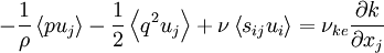
- Transport of kinetic energy in an inhomogeneous field due respectively to the pressure fluctuations, the turbulence itself, and the viscous stresses:
|
| (11) |
- Rate of production of turbulence kinetic energy from the mean flow(gradient):
|
| (12) |
- Rate of dissipation of turbulence kinetic energy per unit mass due to viscous stresses:
|
| (12) |
These terms will be discussed in detail in the succeeding sections, and the role of each examined carefully.
Rate of dissipation of the turbulence kinetic energy
The last term in the equation for the kinetic energy of the turbulence has been identified as the rate of dissipation of the turbulence energy per unit mass; i.e.,
|
| (14) |
It is easy to see that  always, since it is a sum of the average of squared quantities only (i.e.
  ). Also, since it occurs on the right hand side of the kinetic energy equation for the fluctuating motions preceded by a minus sign, it is clear that it can act only to reduce the kinetic energy of the flow. Therefore it causes a negative rate of change of kinetic energy; hence the name dissipation.
Physically, enegry is dissipated because of the work done by the fluctuating viscous stresses in resisting deformation of the fluid material by the fluctuating strain rates; i.e.
|
| (15) |
This reduces to equation 14 only for a Newtonian fluid. In non-Newtonian fluids, protions of this product may not be negative implying that it may not all represent an irrecoverable loss of fluctuating kinetic energy.
It will be shown in the following chapter on stationarity and homogenity that the dissipation of turbulence energy mostly takes place at the smallest turbulence scales, and that those scales can be characterized by so-called Kolmogorov microscale defined by:
|
| (16) |
In atmospheric motions where the length scale for those eddies having the most turbulence energy (and responsible for the Reynolds stress) can be measured in kilometers, typical values of the Kolmogorov microscale range from 0.1 - 10 millimeters. In laboratory flows where the overall scale of the flow is greatly reduced, much smaller values of  are not uncommon. The small size of these dissipative scales greately complicates measurement of energy balances, since the largest measuring dimension must be about equal to twice the Kolmogorov microscale. And it is the range of scales,
  , which makes direct numerical simulation of most interesting flows impossible, since the required number of computational cells is several orders of magnitude greater that
  . This same limitation also affects experiments as well, which must often be quite large to be useful.
One of the consequences of this great separation of scales between those containing the bulk of the turbulence energy and those dissipating it is that the dissipation rate is primarily determined by the large scales and not the small. This is because the viscous scales (which operate on a time scale of  ) dissipate rapidly any energy sent down to them by non-linear processes of scale to scale energy transfer. Thus the overall rate of dissipation is controlled by the rate of energy transfer from the energetic scales, primarily by the non-linear scale-to-scale transfer. This will be discussed later when we consider the energy spactrum. But for now it is important only note that a consequence of this is that the dissipation rate is given approximately as:
|
| (17) |

where  and
and  is an integral length scale. It is easy to remember this relation if you note that the time scale of the energetic turbulent eddies can be estimated as
  . Thus
  can estimated as
  .
.
Sometimes it is convenient to just define the "length scale of the energy containing eddies" (or the pseudo-integral scale) as:
|
| (18) |

Almost always  , but the relation is at most only exact theoretically in the limit of infinite Reynolds number since the constant of proportionality is Reynolds number dependent. The Reynolds number dependence of the ratio
  for grid turbulence is illustrated in Figure 4.1. Many interpret this data to suggest that this ratioapproaches a constant and ignore the scatter. In fact some assume ratio to be constant and even refer to
  though it were the real integral scale. Others argue that the scatter is because of the differing upstream conditions and that the ratio may not be constant at all. It is really hard to tell who is right in the absence of facilities or simulations in which the Reynolds number can vary very much for fixed initial conditions. This all may leave you feeling a bit confused, but that’s the way turbulence is right now. It’s a lot easier to teach if we just tell you one view, but that’s not very good preparation for the future.
Here is what we can say for sure. Only the integral scale, , is a physical length scale, meaning that it can be directly observed in the flow by spectral or correlation measurements (as shown in the following chapters on stationarity and homogenity and homogenous turbulence). The pseudo-integral scale, , on the other hand is simply a definition; and it is only at infinite turbulence Reynolds number that it may have physical significance. But it is certainly a useful
approximation at large, but finite, Reynolds numbers. We will talk about these subtle but important distinctions later when we consider homogeneous flows, but it is especially important when considering similarity theories of turbulence. For
now simply file away in your memory a note of caution about using equation 17 too freely. And do not be fooled by the cute description this provides. It is just that, a description, and not really an explanation of why all this happens — sort
of like the weather man describing the weather. Using equation 18, the Reynolds number dependence of the ratio of the
Kolmorgorov microscale,  , to the pseudo-integral scale, , can be obtained as:
|
| (19) |

Figure 4.1: Ratio of physical integral length scale to pseudo-integral length scale in homogeneous turbulence as function of local Reynolds number,  .
.
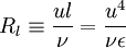
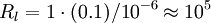
Where the turbulence Reynolds number,  , is defined by:
|
| (20) |
Example: Estimate the Kolmogorov microscale for  and
and  for air and water.
- air For air,
 . Therefore
 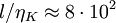 , so
, so 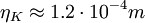 or
or  .
.
- water For water,
 . Therefore
  , so
, so  or
or  .
.
Exercise: Find the dependence on of the time-scale ration between the Kolmorogov microtime and the time scale of the energy-containing eddies. It will also be argued later that these small dissipative scales of motion at very
high Reynolds number tend to be statistically nearly isotropic; i.e., their statistical character is independent of direction. We will discuss some of the implications of isotropy and local isotropy later, but note for now that it makes possible a huge
reduction in the number of unknowns, particularly those determined primarily by the dissipative scales of motion.
Thus the dissipative scales are all much smaller than those characterizing the energy of the turbulent fluctuations, and their relative size decreases with increasing Reynolds number. Note that in spite of this, the Kolmogorov scales all increase with increasing energy containing scales for fixed values of the Reynolds number. This fact is very important in designing laboratory experiments at high turbulence Reynolds number where the finite probe size limits spatial resolution. The rather imposing size of some experiments is an attempt to cope with this problem by increasing the size of the smallest scales, thus making them larger than the resolution limits of the probes being used.
Exercise: Suppose the smallest probe you can build can only resolve  . Also to do an experiment which is a reasonable model of a real engineering flow (like a hydropower plant), you need (for reason that will be clear later) a scale separation of at least
  . If your facility has to be at least a factor of ten larger than (which you estimate as ), what is its smallest dimension?
Kinetic energy of the mean motion and production of turbulence
An equation for the kinetic energy of the mean motion can be derived by a procedure exactly analogous to that applied to the fluctuating motion. The mean motion was shown in 19 in the chapter on Reynolds averaged equations to be given by:
|
| (21) |
![\rho \left[ \frac{\partial U_{i}}{\partial t} + U_{j}\frac{\partial U_{i}}{\partial x_{j}} \right] = -\frac{\partial P}{\partial x_{i}} + \frac{\partial T^{(v)}_{ij}}{\partial x_{j}}- \frac{\partial }{\partial x_{j}}\left(\rho \left\langle u_{i}u_{j} \right\rangle \right)](/W/images/math/f/9/0/f90c4edae80bb7d61d95d9561070998e.png)
By taking the scalar product of this equation with the mean velocity, , we can obtain an equation for the kinetic energy of the mean motion as:
|
| (22) |
![U_{i}\left[ \frac{\partial}{\partial t} + U_{j} \frac{\partial}{\partial x_{j}} \right] U_{i} = - \frac{U_{i}}{\rho} \frac{\partial P}{\partial x_{i}} + \frac{U_{i}}{\rho} \frac{\partial T^{(v)}_{ij} }{\partial x_{j}} - U_{i} \frac{\partial \left\langle u_{i}u_{j} \right\rangle}{\partial x_{j} }](/W/images/math/f/5/d/f5d4730ecd6b791cb354dab3158ee943.png)
Unlike the fluctuating equations, there is no need to average here, since all the terms are already averages.
In exactly the same manner that we rearrannged the terms in the eqyation for the kinetic energy of the fluctuations, we can rearrange the equation for the kinetic energy of the mean flow to obtain:
|
| (23) |
![\begin{matrix}
\left[ \frac{\partial}{\partial t} + U_{j} \frac{\partial}{\partial x_{j}} \right] K = \\
& = & \frac{\partial}{\partial x_{j}} \left\{ - \frac{1}{\rho} \left\langle PU_{i} \right\rangle \delta_{ij} - \frac{1}{2} \left\langle u_{i}u_{j} \right\rangle U_{i} + 2 \nu \left\langle S_{ij} U_{i} \right\rangle \right\} +\\
& + & \left\langle u_{i} u_{j} \right\rangle \frac{\partial U_{i}}{\partial x{j}} - 2 \nu \left\langle S_{ij} S_{ij} \right\rangle \\
\end{matrix}](/W/images/math/3/5/0/350c74568abc450379c1ad8b5d6f6f7e.png)
where
|
| (24) |
The role of all of the terms can immediately be recognized since each term has its counterpart in the equation for the average fluctuating kinetic energy.
Comparison of equations 23 and 6 reveals that the term  appears in the equations for the kinetis energy of BOTH the mean and the fluctuations. There is, however, one VERY important difference. This "production" term has the opposite sign in the equationfor the mean kinetic energy than in that for the mean fluctuating kinetic energy! Therefore, whatever its effect on the kinetic energy of the mean, its effect on the kinetic energy of the fluctuations will be the opposite. Thus kinetic energy can be interchanged between the mean and fluctuating motions. In fact, the only other term involving fluctuations in the equation for the kinetic energy of the mean motion is divergence term; therefore it can only move the kinetic energy of the mean flow from one place to another. Therefore this "production" term provides the only means by which energy can be interchanged between the mean flow and fluctuations.
Understanding the manner in which this energy exchange between mean and fluctuating motions is accomplished represents one of the most challenging problems in turbulence. The overall exchange can be understood by exploiting the analogy which treats  as a stress, the Reynolds stress. The term
  can be thought of as the working of the Reynolds stress against the mean velocity gradient of the flow, exactly as the viscous stresses resist deformation by the instantaneous velocity gradients. This energy expended against the Reynolds stress during deformation by the mean motion ends up in the fluctuating motions, however, while that expended against viscous stresses goes directly to internal energy. As we have already seen, the viscous deformation work from the fluctuating motions (or dissipation) will eventually send this fluctuating kinetic energy on to internal energy as well.
Now, just in case you are not all that clear exactly how the dissipation terms really accomplish this for the instantaneous motion, it might be useful to examine exactly how the above works. We begin by decomposing the mean deformation rate tensor  into its symmetric and antisymmetric parts, exactly as we did for the instantaneous deformation rate tensor in Chapter 3; i.e.,
|
| (25) |
where the mean strain rate  is defined by
|
| (26) |
![S_{ij}=\frac{1}{2}\left[ \frac{\partial U_{i}}{\partial x_{j}} + \frac{\partial U_{j}}{\partial x_{i}} \right]](/W/images/math/1/b/a/1baa28f3f8103315b8311820780a8205.png)
and the mean rotation rate is defined by
|
| (27) |
![\Omega_{ij} = \frac{1}{2}\left[ \frac{\partial U_{i}}{\partial x_{j}} - \frac{\partial U_{j}}{\partial x_{i}} \right]](/W/images/math/9/e/1/9e1326960c808cde3078bf2d87d93a13.png)
Since  is antisymmetric and
  is symmetric, their contraction is zero so it follows that:
|
| (28) |
Equation 28 is an analog to the mean viscous dissipation term given for incompressible flow by:
|
| (29) |
It is easy to show that this term transfers (or dissipates) the mean kinetic energy directly to internal energy, since exactly the same term appears with the opposite sing in the internal energy equations. Moreover, since  always, this is a one-way process and kinetic energy is decreased while internal energy is increased. Hence it can be referred to either as "dissipation" of kinetic energy, or as "production" of internal energy. As surprising as it may seem, this direct dissipation of energy by the mean flow is usually negligible compared to the energy lost to the turbulence through the Reynolds stress term.(Remember, there is a term exactly like this in the kinetic energy equation for the fluctuating motion, but involving only fluctuating quantities; namely
  .) We shall show later that
  . What this means is that most of the energy dissipation is due to the turbulence.
There is a very important difference between equations 28 and 29. Whereas the effect of the viscous stress working against the deformation (in a Newtonian fluid) is always to remove energy from the flow (since always), the effect of the Reynolds stress working against the mean gradient can be of either sign, at least in principle. That is, it can either transfer energy from the mean motion to the fluctuating motion, or vice versa.
Almost always (and especially in situations of engineering importance),  almost always so kinetic energy is removed from the mean motion and added to the fluctuations. Since the term
  usually acts to increase the turbulence kinetic energy, it is usually referred to as the "rate of turbulence energy production", or simply "production".
Now that we have identified how the averaged equations account for the ‘production’ of turbulence energy from the mean motion, it is tempting to think we have understood the problem. In fact, labelling phenomenon is not the same as understanding them. The manner in which the turbulence motions cause this exchange of kinetic energy between the mean and fluctuating motions varies from flow to flow, and is really very poorly understood. Saying that it is the Reynolds stress working against the mean velocity gradient is true, but like saying that money comes from a bank. If we want to examine the energy transfer mechanism in detail we must look beyond the single point statistics, so this will have to be a story for another time.
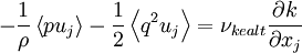
Transport or divergence terms
The overall role of the transport terms is best understood by considering a turbulent flow which is completely confined by rigid walls as in Figure 4.2. First consider only the turbulence transport term. If the volume within the confinement is denoted by  and its bounding surface is
  , then first term on the right-hand side of equation 4.6 for the fluctuating kinetic energy can be integrated over the volume to yield:
|
| (30) |
![\begin{matrix}
& & \int \int \int_{V_{o}} \frac{\partial}{\partial x_{j}} \left[ - \frac{1}{\rho} \left\langle pu_{i} \right\rangle \delta_{ij} - \frac{1}{2} \left\langle q^{2} u_{j} \right\rangle + \nu \left\langle s_{ij} u_{i} \right\rangle \right] dV \\
& = & \int \int_{S_{o}} \left[ - \frac{1}{\rho} \left\langle pu_{i} \right\rangle \delta_{ij} - \frac{1}{2} \left\langle q^{2} u_{j} \right\rangle + \nu \left\langle s_{ij} u_{i} \right\rangle \right] n_{j} dS \\
\end{matrix}](/W/images/math/2/b/c/2bcb570f574505a0555cdaabd6c4caf5.png)
where we have used the divergence theorem - again!
We assumed our enclosure to have rigid walls; therefore the normal component of the mean velocity  must be zero on the surface since there can be no flow through it (the kinematic boundary condition). This immediately eliminates the contributions to the surface integral from the
  and
and  terms. But the last term is zero on the surface also. This can be seen in two ways: either by invoking the no-slip condition which together with the kinematic boundary condition insures that
  is zero on the boundary, or by noting from Cauchy's theorem that
  is the viscous contribution to the normal contact force per unit area on the surface (i.e.,
  ) whose scalar product with must be identically zero since
  is zero. Therefore the entire integral is identically zero and its net contribution to the rate of change of kinetic energy is zero.
Thus the only effect of the turbulence transport terms (in a fixed volume at least) can be to move energy from one place to another, neither creating nor destroying it in the process. This is, of course, why they are collectively called the transport terms. This spatial transport of kinetic energy is accomplished by the acceleration of adjacent fluid due to pressure and viscous stresses (the first and last terms respectively), and by the physical transport of fluctuating kinetic energy by the turbulence itself (the middle term).
This role of these turbulence transport terms in moving kinetic energy around is often exploited by turbulence modellers. It is argued, that on the average, these terms will only act to move energy from regions of higher kinetic energy to lower. Thus a plausible first-order hypothesis is that this "diffusion" of kinetic energy should be proportioned to gradients of the kinetic energy itself. That is,
|
| (31) |
where  is an effective diffusivity like the eddy viscosity discussed earlier. If we use the alternative form of the kinetic energy equation (equation 4.8), there is no need to model the viscous term (since it involves only
  itself). Therefore our model might be:
|
| (32) |
If You think about it, that such a simple closure is worth mentioning at all is pretty amazing. We took 9 unknowns, lumped them together, and replaced their net effect by simple gradient of something we did know (or at least were calculating), . And surprisingly, this simple idea works pretty well in many flows, wspecially if the value of the turbulent viscosity is itself related to other quantities like and  . In fact this simple gradient hypothesis for the turbulence transport terms is at the root of all engineering turbulence models.
There are a couple of things to note about such simple closures though, before getting too enthused about them. First such an assumption rules out a counter-gradient diffusion of kinetic energy which is known to exist in some flows. In such situations the energy appears to flow up the gradient. While this may seem unphysical, remember we only assumed it flowed down the gradient in the first place. This is the whole problem with a plausibility argument. Typically energy does tend to be transported from regions of high kinetic energy to low kinetic energy, but there is really no reason for it always to do so, especially if there are other mechanisms at work. And certainly there is no reason for it to always be true locally, and the gradient of anything is a local quantity.
Let me illustrate this by a simple example. Let's apply a gradient hypothesis to the economy - a plausibility hypothesis if you will By this simple model, money would always flow from the rich who have the most, to the poor who have the least. In fact, as history has shown, in the absence of other forces (like revolutions, beheadings, and taxes) this almost never happens. The rich will always get richer, and the poor poorer. And the reason is quite simple, the poor are usually borrowing, while the rich are loaning - with interest. Naturally there are indidual exceptions and great success stories among the poor. And there are wealthy people who give everything away. But mostly in a completely free economy, the money flows in a counter-gradient manner. So society (and the rich in particular) have a choice - risk beheading and revolution, or find a peaceful means to redistribute the wealth - like taxes. While the general need for the latter is recognized (especially among those who have the least), there is, of course, considerable disagreement of how much tax is reasonable to counter the natural gradient.
Just as the simple eddy viscosity closure for the mean flow can be more generally written as a tensor, so can it be here. In fact the more sophisticated models write it as second or fourth-order tensors. More importantly, they include other gradients in the model so that the gradient of one quantity can influence the gradient of another. Such models can sometimes even accont for counter-gradient behavior. If your study of turbulence takes you into the study of turbulence models watch for these subtle differences among them. And don't let yourself be annoyed or intimidated by their complexity. Instead marvel at the physics behind them, and try to appreciate the wonderful manner in which mathematics has been used to make them properly invariant so you don't have to worry about whether they work in any particular coordinate system. It is all these extra terms that give you reason to hope it might work at all.
The Intercomponent Transfer of Energy
The objective of this section is to examine how kinetic energy produced in one velocity component of the turbulence can be transferred to the other velocity components of the fluctuating motion. This is very important since often energy is transferred from the mean flow to a only a single component of the fluctuating motion. Yet somehow all three components of the kinetic energy end up being about the same order of magnitude. The most common exception to this is very close to surfaces where the normal component is suppressed by the kinematic boundary condition. To understand what is going on, it is necessary to develop even a few more equations; in particular, equations for each component of the kinetic energy. The procedure is almost identical to that used to derive the kinetic energy equation itself.
Consider first the equation for the 1-component of the fluctuating momentum. We can do this by simply setting  and
and  in the equation 35 in the chapter on Reynolds averaged equations , or derive it from scratch by setting the free index in equation 27 in the chapter Reynolds averaged equations
equal to unity (i.e. i=1); i.e.,
in the equation 35 in the chapter on Reynolds averaged equations , or derive it from scratch by setting the free index in equation 27 in the chapter Reynolds averaged equations
equal to unity (i.e. i=1); i.e.,
|
| (33) |
![\left[ \frac{ \partial u_{1}}{\partial t} + U_{j} \frac{ \partial u_{1} }{ \partial x_{j} } \right] = - \frac{1}{ \rho } \frac{ \partial p}{ \partial x_{1} } + \frac{1}{ \rho } \frac{\partial \tau^{(v)}_{1j}}{\partial x_{j}} - \left[ u_{j} \frac{ \partial U_{1} }{ \partial x_{j} } \right] - \left\{ u_{j} \frac{ \partial u_{1} }{ \partial x_{j} } - \left\langle u_{j} \frac{ \partial u_{1} }{ \partial x_{j} } \right\rangle \right\}](/W/images/math/a/7/b/a7ba5b7796dfe0e7385962bb7234d269.png)
Multiplying this equation by  , averaging, and rearranging the pressure-velocity gradient term using the chain rule for products yields:
1-component
|
| (34) |
![\begin{matrix}
\left[ \frac{ \partial }{ \partial t} + U_{j} \frac{ \partial }{ \partial x_{j} } \right] \frac{1}{2} \left\langle u^{2}_{1}\right\rangle = \\
& = & \left\langle p \frac{\partial u_{1}}{\partial x_{1} } \right\rangle + \\
& + & \frac{ \partial }{ \partial x_{j}} \left\{ -\frac{1}{\rho} \left\langle p u_{1} \right\rangle \delta_{1j} - \frac{1}{2} \left\langle u^{2}_{1} u_{j} \right\rangle + 2 \nu \left\langle s_{1j} u_{1} \right\rangle \right\} - \\
& - & \left\langle u_{1} u_{j} \right\rangle \frac{\partial U_{1}}{ \partial x_{j}} - 2 \nu \left\langle s_{1j} s_{1j} \right\rangle \\
\end{matrix}](/W/images/math/0/7/7/077fc3676e92ee0b97f0314032b625aa.png)
All of the terms except one look exactly like the their counterparts in equation 6 for the average of the total fluctuating kinetic energy. The single exception is the first term on the right-hand side which is the contribution from the pressure-strain rate. This will be seen to be exactly the term we are looking for to move energy among the three components.
Similar equations can be derived for the other fluctuating components with the result that
2-component
|
| (35) |
![\begin{matrix}
\left[ \frac{ \partial }{ \partial t} + U_{j} \frac{ \partial }{ \partial x_{j} } \right] \frac{1}{2} \left\langle u^{2}_{2}\right\rangle = \\
& = & \left\langle p \frac{\partial u_{2}}{\partial x_{2} } \right\rangle + \\
& + & \frac{ \partial }{ \partial x_{j}} \left\{ -\frac{1}{\rho} \left\langle p u_{2} \right\rangle \delta_{2j} - \frac{1}{2} \left\langle u^{2}_{2} u_{j} \right\rangle + 2 \nu \left\langle s_{2j} u_{2} \right\rangle \right\} - \\
& - & \left\langle u_{2} u_{j} \right\rangle \frac{\partial U_{2}}{ \partial x_{j}} - 2 \nu \left\langle s_{2j} s_{2j} \right\rangle \\
\end{matrix}](/W/images/math/3/5/f/35fb18242d4e7d960506f9be7de1f628.png)
and
3-component
|
| (36) |
![\begin{matrix}
\left[ \frac{ \partial }{ \partial t} + U_{j} \frac{ \partial }{ \partial x_{j} } \right] \frac{1}{2} \left\langle u^{2}_{3}\right\rangle = \\
& = & \left\langle p \frac{\partial u_{3}}{\partial x_{3} } \right\rangle + \\
& + & \frac{ \partial }{ \partial x_{j}} \left\{ -\frac{1}{\rho} \left\langle p u_{3} \right\rangle \delta_{3j} - \frac{1}{2} \left\langle u^{2}_{3} u_{j} \right\rangle + 2 \nu \left\langle s_{3j} u_{3} \right\rangle \right\} - \\
& - & \left\langle u_{3} u_{j} \right\rangle \frac{\partial U_{3}}{ \partial x_{j}} - 2 \nu \left\langle s_{3j} s_{3j} \right\rangle \\
\end{matrix}](/W/images/math/0/4/e/04e9695a18b70d06a1e8625a55b18015.png)
Note that in each equation a new term involving a pressure-strain rate has appeared as the first term on the right-hand side. It is straightforward to show that these three equations sum to the kinetic energy equation given by equation 6, the extra pressure terms vanishing for the incompressible flow assumed here. In fact, the vanishing of the pressure-strain rate terms when the three equations are added together gives a clue as to their role. Obviously they can neither create nor destroy kinetic energy, only move it from one component of the kinetic energy to another.
The precise role of the pressure terms can be seen by noting that incompressibility implies that:
|
| (37) |
It follows immediately that:
|
| (38) |
![\left\langle p \frac{\partial u_{1} }{ \partial x_{1} } \right\rangle = - \left[ \left\langle p \frac{\partial u_{2} }{ \partial x_{2} } \right\rangle + \left\langle p \frac{\partial u_{3} }{ \partial x_{3} } \right\rangle \right]](/W/images/math/0/4/9/049ad8f48a76421d28309557b38eb3d4.png)
Thus equation 34 can be rewritten as:
|
| (39) |
![\begin{matrix}
\left[ \frac{ \partial }{ \partial t} + U_{j} \frac{ \partial }{ \partial x_{j} }\right] \frac{1}{2} \left\langle u^{2}_{1} \right\rangle = \\
= & - & \left[ \left\langle p \frac{\partial u_{2} }{ \partial x_{2} } \right\rangle + \left\langle p \frac{\partial u_{3} }{ \partial x_{3} } \right\rangle \right] + \\
& + & \frac{ \partial }{ \partial x_{j}} \left\{ -\frac{1}{\rho} \left\langle p u_{1} \right\rangle \delta_{1j} - \frac{1}{2} \left\langle u^{2}_{1} u_{j} \right\rangle + 2 \nu \left\langle s_{1j} u_{1} \right\rangle \right\} - \\
& - & \left\langle u_{1} u_{j} \right\rangle \frac{\partial U_{1}}{ \partial x_{j}} - 2 \nu \left\langle s_{1j} s_{1j} \right\rangle \\
\end{matrix}](/W/images/math/e/3/0/e309d1d7a25835491ffb506b89edcf87.png)
Comparison of equation 39 with equations 35 and 36 make it immediately apparent that the pressure strain rate terms act to exchange energy between components of the turbulence. If  and
and  are both positive, then energy is removed from the 1-equation and put into the 2- and 3-equations since the same terms occur with opposite sign. O vice versa.
The role of the pressure strain rate terms can best be illustrated by looking at simple example. Consider a simple homogeneous shear flow in which  and in which the turbulence is homogeneous. For this flow, the assumption of homogeneity insures that all terms involving gradients of average quantities vanish (except for
  ). This leaves only the pressure-strain rate, production and dissipation terms; therefore equations 35, 36, 39 reduce to:
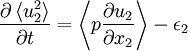
1-component
|
| (40) |
![\frac{\partial \left\langle u^{2}_{1} \right\rangle}{ \partial t} = - \left[ \left\langle p \frac{ \partial u_{2} }{ \partial x_{2} } \right\rangle + \left\langle p \frac{ \partial u_{3} }{ \partial x_{3} } \right\rangle \right] - \left\langle u_{1} u_{2} \right\rangle \frac{ \partial U_{1} }{ \partial x_{2}} - \epsilon_{1}](/W/images/math/9/b/d/9bd94063effe39030c39dd7bbca7c0f7.png)
2-component
|
| (41) |
3-component
|
| (42) |

where
|
| (43) |
|
| (44) |
|
| (45) |
It is immediately apparent that only  can receive energy from the mean flow because only the first equation has a non-zero production term.
Now let's further assume that the smallest scales of the turbulece can be assumed to be locally isotropic. While not always true, this is a pretty good approximation for high Reynolds number flows. (Note that it might be exactly true in many flows in the limit of infinite Reynolds number, at least away from walls.) Local isotropy implies that the component dissipation rates are equal; i.e.,  . But where does the energy in the 2 and 3-components come from? Obviously the pressure-strain-rate terms must act to remove energyfrom the 1-component and redistribute it to the others.
As the preceding example makes clear, the role of the pressure-strain-rate terms is to attempt to distribute the energy among the various components of the turbulence. In the absence of other influences, they are so successful that the dissipation by each component is almost equal, at least at high turbulence Reynolds numbers. In fact, because of the energy re-distribution by the the pressure strain rate terms, it is uncommon to find a turbulent shear flow away from boundaries where the kinetic energy of the turbulence components differ by more than 30-40%, no matter which component gets the energy from the mean flow.
* *
Credits
This text was based on "Lectures in Turbulence for the 21st Century" by Professor William K. George, Professor of Turbulence, Chalmers University of Technology, Gothenburg, Sweden.