Jacobi method
From CFD-Wiki
(Added an example calculation here, too) |
|||
| Line 1: | Line 1: | ||
| - | + | The Jacobi method is an algorithm in linear algebra for determining the solutions of a system of linear equations with largest absolute values in each row and column dominated by the diagonal element. Each diagonal element is solved for, and an approximate value plugged in. The process is then iterated until it converges. This algorithm is a stripped-down version of the Jacobi transformation method of matrix diagonalization. The method is named after German mathematician [http://en.wikipedia.org/wiki/Carl_Gustav_Jakob_Jacobi Carl Gustav Jakob Jacobi]. | |
We seek the solution to set of linear equations: <br> | We seek the solution to set of linear equations: <br> | ||
| Line 16: | Line 16: | ||
</math> | </math> | ||
| - | Note that the computation of <math>\phi^{(k+1)}_i</math> requires each element in <math>\phi^{(k)}</math> except itself. Then, unlike in the [[Gauss-Seidel method]], we can't overwrite <math>\phi^{(k)}_i</math> with <math>\phi^{(k+1)}_i</math>, as that value will be needed by the rest of the computation. This is the most meaningful difference between the Jacobi and Gauss-Seidel methods. The minimum | + | Note that the computation of <math>\phi^{(k+1)}_i</math> requires each element in <math>\phi^{(k)}</math> except itself. Then, unlike in the [[Gauss-Seidel method]], we can't overwrite <math>\phi^{(k)}_i</math> with <math>\phi^{(k+1)}_i</math>, as that value will be needed by the rest of the computation. This is the most meaningful difference between the Jacobi and Gauss-Seidel methods. The minimum amount of storage is two vectors of size <math>n</math>, and explicit copying will need to take place. |
== Algorithm == | == Algorithm == | ||
| - | + | Choose an initial guess <math>\phi^{0}</math> to the solution <br> | |
| - | : for k := 1 step 1 | + | : for k := 1 step 1 until convergence do <br> |
:: for i := 1 step until n do <br> | :: for i := 1 step until n do <br> | ||
::: <math> \sigma = 0 </math> <br> | ::: <math> \sigma = 0 </math> <br> | ||
| Line 34: | Line 34: | ||
==Convergence== | ==Convergence== | ||
| - | + | The method will always converge if the matrix A is strictly or irreducibly diagonally dominant. Strict row diagonal dominance means that for each row, the absolute value of the diagonal term is greater than the sum of absolute values of other terms: | |
| + | |||
:<math>\left | a_{ii} \right | > \sum_{i \ne j} {\left | a_{ij} \right |} </math> | :<math>\left | a_{ii} \right | > \sum_{i \ne j} {\left | a_{ij} \right |} </math> | ||
| - | |||
| - | + | The Jacobi method sometimes converges even if this condition is not satisfied. It is necessary, however, that the diagonal terms in the matrix are greater (in magnitude) than the other terms. | |
== Example Calculation == | == Example Calculation == | ||
| Line 152: | Line 152: | ||
| - | ==External | + | ==External links== |
| - | *[http://en.wikipedia.org/wiki/Jacobi_method Wikipedia | + | *[http://www.math-linux.com/spip.php?article49 Jacobi method from www.math-linux.com] |
| + | *[http://mathworld.wolfram.com/JacobiMethod.html Jacobi Method at Math World] | ||
| + | *[http://en.wikipedia.org/wiki/Jacobi_method Jacobi method at Wikipedia] | ||
Revision as of 10:08, 12 May 2007
The Jacobi method is an algorithm in linear algebra for determining the solutions of a system of linear equations with largest absolute values in each row and column dominated by the diagonal element. Each diagonal element is solved for, and an approximate value plugged in. The process is then iterated until it converges. This algorithm is a stripped-down version of the Jacobi transformation method of matrix diagonalization. The method is named after German mathematician Carl Gustav Jakob Jacobi.
We seek the solution to set of linear equations:

In matrix terms, the definition of the Jacobi method can be expressed as :
![\phi^{(k+1)} = D^{ - 1} \left[\left( {L + U} \right)\phi^{(k)} + b\right]](/W/images/math/2/5/1/251a2f655111e185ad6346ba43ad3117.png)
where  ,
,  , and
, and  represent the diagonal, lower triangular, and upper triangular parts of the coefficient matrix
  and
and  is the iteration count. This matrix expression is mainly of academic interest, and is not used to program the method. Rather, an element-based approach is used:
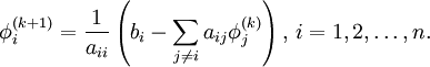
Note that the computation of  requires each element in
  except itself. Then, unlike in the Gauss-Seidel method, we can't overwrite
  with , as that value will be needed by the rest of the computation. This is the most meaningful difference between the Jacobi and Gauss-Seidel methods. The minimum amount of storage is two vectors of size
  , and explicit copying will need to take place.
Contents |
Algorithm
Choose an initial guess  to the solution
- for k := 1 step 1 until convergence do
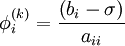
- for i := 1 step until n do
-

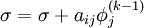
- for j := 1 step until n do
- if j != i then
-
- end if
- if j != i then
- end (j-loop)
-
-
- end (i-loop)
- check if convergence is reached
- for i := 1 step until n do
- end (k-loop)
Convergence
The method will always converge if the matrix A is strictly or irreducibly diagonally dominant. Strict row diagonal dominance means that for each row, the absolute value of the diagonal term is greater than the sum of absolute values of other terms:
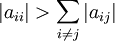
The Jacobi method sometimes converges even if this condition is not satisfied. It is necessary, however, that the diagonal terms in the matrix are greater (in magnitude) than the other terms.
Example Calculation
As with Gauss-Seidel, Jacobi iteration lends itself to situations in which we need not explicitly represent the matrix. Consider the simple heat equation problem
![\nabla^2 T(x) = 0,\ x\in [0,1]](/W/images/math/6/8/1/681af3c6083368314f689c744b5b198c.png)
subject to the boundary conditions  and
and  . The exact solution to this problem is
  . The standard second-order finite difference discretization is
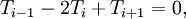
where  is the (discrete) solution available at uniformly spaced nodes (see the Gauss-Seidel example for the matrix form). For any given for
  , we can write
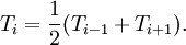
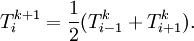
Then, stepping through the solution vector from  to
to  , we can compute the next iterate from the two surrounding values. For a proper Jacobi iteration, we'll need to use values from the previous iteration on the right-hand side:
The following table gives the results of 10 iterations with 5 nodes (3 interior and 2 boundary) as well as  norm error.
| Iteration |  |  |  |  |  | error
|
|---|---|---|---|---|---|---|
| 0 | 0.0000E+00 | 0.0000E+00 | 0.0000E+00 | 0.0000E+00 | 1.0000E+00 | 1.0000E+00 |
| 1 | 0.0000E+00 | 0.0000E+00 | 0.0000E+00 | 5.0000E-01 | 1.0000E+00 | 6.1237E-01 |
| 2 | 0.0000E+00 | 0.0000E+00 | 2.5000E-01 | 5.0000E-01 | 1.0000E+00 | 4.3301E-01 |
| 3 | 0.0000E+00 | 1.2500E-01 | 2.5000E-01 | 6.2500E-01 | 1.0000E+00 | 3.0619E-01 |
| 4 | 0.0000E+00 | 1.2500E-01 | 3.7500E-01 | 6.2500E-01 | 1.0000E+00 | 2.1651E-01 |
| 5 | 0.0000E+00 | 1.8750E-01 | 3.7500E-01 | 6.8750E-01 | 1.0000E+00 | 1.5309E-01 |
| 6 | 0.0000E+00 | 1.8750E-01 | 4.3750E-01 | 6.8750E-01 | 1.0000E+00 | 1.0825E-01 |
| 7 | 0.0000E+00 | 2.1875E-01 | 4.3750E-01 | 7.1875E-01 | 1.0000E+00 | 7.6547E-02 |
| 8 | 0.0000E+00 | 2.1875E-01 | 4.6875E-01 | 7.1875E-01 | 1.0000E+00 | 5.4127E-02 |
| 9 | 0.0000E+00 | 2.3438E-01 | 4.6875E-01 | 7.3438E-01 | 1.0000E+00 | 3.8273E-02 |
| 10 | 0.0000E+00 | 2.3438E-01 | 4.8438E-01 | 7.3438E-01 | 1.0000E+00 | 2.7063E-02 |