Rhie-Chow interpolation
From CFD-Wiki
(Difference between revisions)
| (7 intermediate revisions not shown) | |||
| Line 1: | Line 1: | ||
we have at each cell descretised equation in this form, <br> | we have at each cell descretised equation in this form, <br> | ||
:<math> a_p \vec v_P = \sum\limits_{neighbours} {a_l } \vec v_l - \frac{{\nabla p}}{V} </math> ; <br> | :<math> a_p \vec v_P = \sum\limits_{neighbours} {a_l } \vec v_l - \frac{{\nabla p}}{V} </math> ; <br> | ||
| - | we have <br> | + | For continuity we have <br> |
| - | :<math> \ | + | :<math> \sum\limits_{faces} \left[ {\frac{1}{{a_p }}H} \right]_{face} = \sum\limits_{faces} \left[ {\frac{1}{{a_p }}\frac{{\nabla p}}{V}} \right]_{face} </math> <br> |
| - | + | where <br> | |
| - | : | + | :<math> H = \sum\limits_{neighbours} {a_l } \vec v_l </math> <br> |
| - | + | ||
| - | + | ||
| - | + | ||
| - | + | ||
| - | + | ||
| - | + | ||
| - | + | ||
| - | + | ||
| - | + | ||
| - | + | This interpolation of variables H and <math> {\nabla p} </math> based on coefficients <math> a_p </math> for [[Velocity-pressure coupling | pressure velocity coupling ]] is called <b>Rhie-Chow interpolation</b>. | |
| + | |||
| + | the Rhie-Chow interpolation is the same as adding a pressure term, which is proportional to a third derivative of the pressue | ||
| + | |||
| + | ---- | ||
| + | <i> Return to: <br> | ||
| + | # [[Numerical methods | Numerical Methods]] | ||
| + | # [[Solution of Navier-Stokes equation]] | ||
| + | </i> | ||
Latest revision as of 06:14, 27 August 2012
we have at each cell descretised equation in this form,
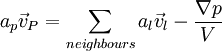 ;
;
For continuity we have
![\sum\limits_{faces} \left[ {\frac{1}{{a_p }}H} \right]_{face} = \sum\limits_{faces} \left[ {\frac{1}{{a_p }}\frac{{\nabla p}}{V}} \right]_{face}](/W/images/math/8/7/1/8716a0f2e3b6892c158df26a9c5b8c67.png)
where
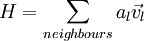
This interpolation of variables H and  based on coefficients
  for pressure velocity coupling is called Rhie-Chow interpolation.
the Rhie-Chow interpolation is the same as adding a pressure term, which is proportional to a third derivative of the pressue
Return to: