Two phase flow
From CFD-Wiki
(→Eddy Interaction Model) |
(→Eddy Interaction Model) |
||
| Line 58: | Line 58: | ||
The fluid fluctuating velocity is randomly sampled with a Gaussian PDF of mean and variance that are deduced from turbulence model, as previously described. | The fluid fluctuating velocity is randomly sampled with a Gaussian PDF of mean and variance that are deduced from turbulence model, as previously described. | ||
| - | [[Image:Eddy interaction.JPG|thumb|Eddy Interation Model]] | + | [[Image:Eddy interaction.JPG|thumb|Eddy Interation Model (Graham & James 1996)]] |
Revision as of 10:36, 7 November 2007
Contents |
Introduction
article in progress
Importance of two phase flow in industrial configurations
Two phase flow phenomena occur in various industrial application in all fluid mechanics application fiels. Aerospace, automotive, nuclear applications, etc. In all this domain, prediction of two phase behaviour is important. Prediction of liquid spray in an internal combustion engine should enable us to have a better control on combustion process and then to reduce pollutant emissions. Controlling water - steam equilibrium in a coller system enable to prevent from industrial accident, de-icing/anti-icing of aircraft on the ground etc. Any other examples can be quoted here.
Overview of the different available approach
Two main family can be distinguished to model two phase flow, depending of the two phase configuration approach. In case of dispersed configuration a lagrangian approach is suitable. Such an approach consists in following dropplets (or bubbles) during then movement. This is done by applying external force on the particle and solving acceleration, then velocity and finally position. On the other hand, two phase flow can be solve with an eulerien approach. As in all eulerian framework, this approach consists in considering inlet and outlet flux in a given volume. In such an eulerian approach, two family can be distinguished : Mixture model and Two fluids model, those two approach will be detailed in corresponding section bellow.
Lagrangian dispersed two-phase flow modelling
The main goal in Lagrangien approaches is to statiscally particle history in given flow fields. The starting point in Lagrangien approach is the fundamental law of dynamics:
Where  stands for the resulting force on the particle.
Resolution of these equations requires the knowledge of the instantaneous velocity of the fluid at particle position. The problem is thus to track fluid particles along the discrete particle trajectory.
A fluid particle instantaneously owns the velocity of the surrounding fluid and the simulation of its trajectory relies on a quite simple equation such as:

The instantaneous fluid velocity  is decomposed into a mean part which is known (from turbulence model prediction) and a fluctuating part
  .
So generating fluctuating part of the fluid velocity is the core of the problem.
Generation of the fluid particle velocity fluctuations is based on a Gaussian PDF for the fluid velocities, but different random schemes can then be used to guess the fluid velocity, which are characterized by the underlying fluid Lagrangian correlation function
  .
.

The first approach was proposed by Gosman and Ioannides (1981) and has been called “eddy life time”. Each fluid velocity fluctuation is kept constant on a time step which is equal to the Lagrangian integral time scale  . The resulting Lagrangian correlation function is linearly decreasing from 1 to 0 in a time delay equal to
  :
:

A first extension has been proposed by Ormancey & Martinon (1984) and is commonly used in the Lagrangian community. In that scheme, a Poisson distribution of the time interval is introduced: each fluid velocity fluctuation is kept constant until a random number (uniformly distributed between 0 and 1) is smaller than  . The resulting fluid Lagrangian correlation function is exponentially decreasing from 1 to 0:

Later, Desjonqueres (1987) proposed a process which can handle any given correlation function. This can be done through a correlation matrix, as described by Berlemont et al (1990) or Boughattas et al. (2006). Moreover, Desjonqueres (1987) introduced the Frenkiel family of correlation function (1948) which are defined by:
![{R_{fl}(\tau)}=exp[\frac{-\tau}{(m^2+1)\tau_l}] cos[\frac{m\tau}{(m^2+1)\tau_l}]](/W/images/math/a/a/6/aa64bfd8d6f904364d7ef6bf12d2896a.png)
Where m is a loop parameter, giving the exponential decrease for m=0. Let us note that this function presents negative loops and m=1 is the value used by Picart (1981) during confrontations of simulations with the experimental data.
Eddy Interaction Model
Historically, the first approach which has been developed and widely used in engineering calculations is the Eddy Interaction Model, first described by Gosman and Ioannides (1981). In the Eddy Interaction Model, the discrete particle is assumed to interact with a succession of eddies. Each eddy is characterized by a velocity (fluctuating), a time scale (lifetime) and a length scale (size). The fluid fluctuating velocity is randomly sampled with a Gaussian PDF of mean and variance that are deduced from turbulence model, as previously described.
The eddy life time and the eddy length scale can be estimated from the local turbulence properties and defined by:


The time  for a particle to cross the eddy is calculated from the particle velocity (at the beginning of the time step) and the length scale
  .
.
![{t_{c}}=-\tau_{p}ln[ 1- \frac{l_{e}}{\tau_{p} {\left|\vec u_f-\vec u_p \right|}}]](/W/images/math/0/8/b/08b7239e9ca63e74374305fc55098766.png)
The particle is assumed to interact with the eddy for a time which is the minimum of the eddy life time and the eddy transit time  . During that interaction the fluid fluctuating velocity is kept constant and the discrete particle is moved with respect to its equation of motion. Then a new fluctuating fluid velocity is sampled and the process is repeated.
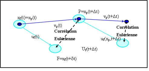
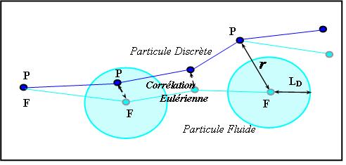
The Correlated-Time Model is similar to the Eddy Interaction Model in a sense that the focus is also to solve the particle trajectory, the difference lies in how the fluctuating fluid velocity is determined along the particle trajectory. The Correlated-Time Model is based on the simultaneous realization of a fluid trajectory and a particle trajectory. The fluid velocity is transferred from the fluid position to the particle position with respect to Eulerian correlation. This process is carried out until the discrete particle leaves a correlation domain defined around the fluid particle.
Mixture model for two phase flow
Basics of the mixture model
MAC approach
VOF method
Eulerian Two fluids approach
Basics of the two fluids approach
Interfacial exchange closures
Turbulence modelling in such a context
Conclusion
References
- Berlemont A., Desjonqueres PH., Guesbet G. (1990), "Particle Lagrangian simulation in turbulent Flows", Int. J. Multiphase Flow, 16-1, pp 19-34.
- Boughattas N., Gazzah M. H., Said R. (2006), "Effects of a co-flow on particles or droplets dispersion and on droplets vaporization in turbulent air flow", ICAMEM2006, Hammamet, Tunisia.
- Boughattas N., Gazzah M. H., Said R. (2007), "Lagrangian prediction of particulate two-phase flow", Fifth Mediterranean Combustion Symposium, Monastir, Tunisia.
- Desjonqueres PH. (1987), "Modélisation Lagrangienne du comportement de particules discrètes en écoulement turbulent", Thèse de doctorat, Faculté des Sciences de L’université de Rouen, France.
- Frenkiel F.N. (1948), "Etude statistique de la turbulence - fonctions spectrales et coefficients de corrélation", Rapport technique. ONERA n° 34.
- Gosman A. D., Ionnides I. E. (1981), "Aspects of computer simulation of liqued fuelled combustors", AIAA aerospace sciences meeting, paper 81-0323, St.louis,MO.
- Ormancey A., Martinon A. (1984), "Prediction of particle dispersion in turbulent flows", Physico-Chemical Hydrodynamics, 5-314, pp 229-244.
- Picart A., Berlement A., Guesbet G. (1986), "Modelling and predicting turbulence fields and the dispersion of discrete particles transported by turbulent Flows", Int. J. Heat and Mass Transfer, 12-2, pp 237-261.


