Diffusion term
From CFD-Wiki
Contents |
Discretisation of the diffusion term
Description
For a general control volume (orthogonal, non-orthogonal), the discretization of the diffusion term can be written in the following form
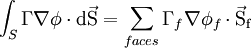
where
- S denotes the surface area of the control volume
 denotes the area of a face for the control volume
As usual, the subscript f refers to a given face. The figure below describes the terminology used in the framework of a general non-orthogonal control volume

A general non-orthogonal control volume
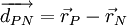
If  and
and  are position vector of centroids of cells P and N respectively. Then, we define
We wish to approaximate the diffusive flux 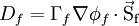 at the face.
Approach 1
A first approach is to use a simple expression for estimating the gradient of a scalar normal to the face.
![D_f = \Gamma _f \nabla \phi _f \cdot \vec S_f = \Gamma _f \left[ {\left( {\phi _N - \phi _P } \right)\left| {{{\vec S_f} \over {\overrightarrow{d_{PN}}}}} \right|} \right]](/W/images/math/2/2/f/22f7fe72fd16546ff2d65bf48adf7a35.png)
where  is a suitable face average.
This approach is not very good when the non-orthogonality of the faces increases. If this is the case, it is advisable to use one of the following approaches.
Approach 2
We define the vector

giving us the expression:
![D_f = \Gamma _f \nabla \phi _f \cdot{\rm{\vec S_f = }}\Gamma _{\rm{f}} \left[ {\left( {\phi _N - \phi _P } \right)\vec \alpha \cdot {\rm{\vec S_f + }}\bar \nabla \phi_f \cdot {\rm{\vec S_f - }}\left( {\bar \nabla \phi_f \cdot {\overrightarrow{d_{PN}}}} \right)\vec \alpha \cdot {\rm{\vec S_f}}} \right]](/W/images/math/7/c/f/7cf1e0cce420c5d8f260ea5c7f3340ff.png)
where  and are suitable face averages.
Orthogonal correction approaches
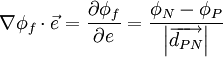
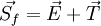
In non-orthogonal grids, the gradient direction that will yield an expression involving the values at the neighboring control volumes will have to be along the line joining the centroids of the two control volumes. If this direction has a unit vector denoted by  then, by definition

then the gradient in the direction of can be written as
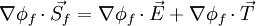
If the surface vector  is written as the summation of two vectors
  and
and 
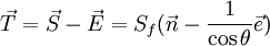
where is in the direction joining the centroids of the two control volumes, we will then be able to express the diffusive flux in terms of the neighboring control volumes plus an additional correction. This is done as follows
 .... (where E is the magnitude of
At the outset, one obtains
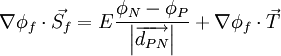
The first term in the above equation can be thought of as the orthogonal contribution to the diffusive flux, while the second term represents the non-orthogonal effects. At this point, the vector has not been defined yet. There are three main methods to define this vector.
Minimum correction
In the minimum correction approach, the vectors are defined as
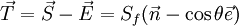

Minimum Correction Approach
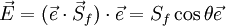
Orthogonal correction
In the orthogonal correction approach, the vectors are defined as

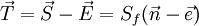

Orthogonal Correction Approach
Over relaxed correction
Finally, in the over relaxed approach, we define
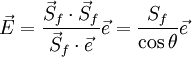

Over Relaxed Correction Approach
References
- Ferziger, J.H. and Peric, M. (2001), Computational Methods for Fluid Dynamics, ISBN 3540420746, 3rd Rev. Ed., Springer-Verlag, Berlin..
- Hrvoje, Jasak (1996), "Error Analysis and Estimation for the Finite Volume Method with Applications to Fluid Flows", PhD Thesis, Imperial College, University of London (download).
- Darwish, Marwan (2003), "CFD Course Notes", Notes, American University of Beirut.
- Saad, Tony (2005), "Implementation of a Finite Volume Unstructured CFD Solver Using Cluster Based Parallel Computing", Thesis, American University of Beirut.
Return to Numerical Methods