Introduction to turbulence/Free turbulent shear flows
From CFD-Wiki
(→Implications of the Reynolds stress equations) |
(→Implications of the Reynolds stress equations) |
||
| Line 609: | Line 609: | ||
<table width="70%"><tr><td> | <table width="70%"><tr><td> | ||
:<math> | :<math> | ||
| - | + | U \frac{\partial \left\langle uv \right\rangle}{ \partial x} + V \frac{\partial \left\langle uv \right\rangle}{ \partial y} = | |
</math> | </math> | ||
| - | </td><td width="5%">( | + | </td><td width="5%">(46)</td></tr></table> |
| - | + | ||
| - | + | ||
<table width="70%"><tr><td> | <table width="70%"><tr><td> | ||
:<math> | :<math> | ||
| - | + | = \left\langle p \left( \frac{ \partial u}{ \partial y} + \frac{ \partial v}{ \partial x} \right) \right\rangle + \frac{ \partial }{ \partial y} \left\{ - \left\langle u v^{2} \right\rangle \right\} - \left\langle v^{2} \right\rangle \frac{ \partial U}{ \partial y} | |
</math> | </math> | ||
| - | </td><td width="5%">( | + | </td><td width="5%">(46)</td></tr></table> |
Revision as of 15:01, 13 March 2011
Contents |
Introduction
Free shear flows are inhomogeneous flows with mean velocity gradients that develop in the absence of boundaries. Turbulent free shear flows are commonly found in natural and engineering environments. The jet of of air issuing from one's nostrils or mouth upon exhaling, the turbulent plume from a smoldering cigarette, and the buoyant jet issuing from an erupting volcano - all illustrate both the omnipresence of free turbulent shear flows and the range of scales of such flows in the natural environment. Examples of the multitude of engineering free shear flows are the wakes behind moving bodies and the exhausts from jet engines. Most combustion processes and many mixing processes involve turbulent free shear flows.
Free shear flows in the real world are most often turbulent. Even if generated as laminar flows, they tend to become turbulent much more rapidly than the wall-bounded flows which we will discuss later. This is because the three-dimensional vorticity necessary for the transition to turbulence can develop much more rapidly in the absence of walls that inhibit the qrowth velocity components normal to them.
The tendency of free shear flows to become and remain turbulent can be greatly modified by the presence of density gradients in the flow, especially if gravitational effects are also important. Why this is the case can easily be seen by examining the vorticity equation for such flows in the absence of viscosity,
|
| (1) |
![\left[ \frac{ \partial \omega_{i} }{ \partial t } + \tilde{u_{j}} \frac{ \partial \tilde{\omega_{i} } }{ \partial x_{j}} \right] = \tilde{\omega_{j} } \frac{ \partial \tilde{u_{i}} }{ \partial x_{j} } + \epsilon_{ijk} \frac{ \partial \tilde{ \rho } }{ \partial x_{j} } \frac{ \partial \tilde{p} }{ \partial {x_{k} } }](/W/images/math/6/f/0/6f02543bf32edff708a67c788f0dd077.png)
The last term can act to either increase or decrease vorticity production but only in non-barotropic flows. (Recall that a barotropic flow is one in which the gradients of density and pressure are co-linear, because the density is a function of the pressure only). For example, in the vertically-oriented buoyant plume generated by exhausting a lighter fluid into heavier one, the principal density gradient is across the flow and thus perpendicular to the gravitational force which is the principal contributor to the pressure gradient. As a consequence the turbulent buoyant plume develops much more quickly than its uniform density counterpart, the jet. On the other hand, horizontal free shear flows in a stably stratified environment (fluid density decreases with height) can be quickly suppressed since the density and pressure gradients are in opposite directions.
Free turbulent shear flows are distinctly different from the homogeneous shear flows. In a free turbulent shear flow, the vortical fluid is patially confined and is separated from the surrounding fluid by an interface, the turbulent-nonturbulent interface (also known as the ”Corrsin superlayer” after itself discoverer). The turbulent/non-turbulent interface has a thickness which is characterized by the Kolmogorov microscale, thus its characterization as an interface is appropriate. The actual shape of the interface is random and it is severely distorted by the energetic turbulent processes which take place below it, with the result that at any given location the turbulence can be highly intermittent. This means that at a given location, it is sometimes turbulent, sometimes not.
It should not be inferred from the above that the non-turbulent fluid outside the superlayer is quiescent. Quite the opposite is true since the motion of the fluid at the interface produces motions in the surrounding stream just as would the motions of a solid wall. Alternately, the flow outside the interface can be viewed as being “induced” by the vortical motions beneath it. It is easy to show that these induced motions are irrotational. Thus since these random motions of the outer flow have no vorticity, they can not be considered turbulent.
Figure 7.1 shows records of the velocity versus time at a number of locations in the mixing layer of a round jet. When turbulent fluid passes the probes, the velocity signals are characterized by bursts of activity. The smooth undulations between the bursts are the irrotational fluctuations induced by the turbulent vorticity on the other side of the interface. Note that near the center of the mixing layer where the shear is a maximum, the flow is nearly always turbulent while it becomes increasingly intermittent as one proceeds away from the region of maximum production of turbulence energy. This increasing intermittency toward the outer edge is a characteristic of all free shear flows, and is an indication of the fact that the turbulent/non-turbulent interface is constantly changing its position.
One of the most important features of free shear flows is that the amount of fluid which is turbulent is continuously increased by a process known as entrainment. No matter how little fluid is in the flow initially, the turbulent part of the flow will continue to capture new fluid by entrainment as it evolves. The photograph of an air jet in Figure 1.2 illustrates this phenomenon dramatically. The mass flow of the jet increases at each cross-section due to entrainment. Entrainment is not unique to turbulent flows, but is also an important haracteristic of laminar flow, even though the actual mechanism of entrainment is quite different.
There are several consequences of entrainment. The first and most obvious is that free shear flows continue to spread throughout their lifetime. (That such is the case for the air jet of Figure 7.1 is obvious). A second consequence of entrainment is that the fluid in the flow is being continuously diluted by the addition of fluid from outside it. This is the basis of many mixing processes, and without such entrainment our lives would be quite different. A third consequence is that it will never be possible to neglect the turbulent transport terms in the dynamical equations, at least in the directions in which the flow is spreading. This is because the dilution process has ensured that the flow can never reach homogeneity since it will continue to entrain and spread through its lifetime (Recall that the transport terms were identically zero in homogeneous flows). Thus in dealing with free shear flows, all of the types of terms encountered in the turbulence kinetic energy equation of Chapter 4 must be dealt with — advection, dissipation, production, and turbulent transport.
Turbulent free shear flows have another distinctive feature in that they very often give rise to easily recognizable large scale structures or eddies. Figure 1.2 also illustrates this phenomenon, and coherent patterns of a scale equal to the lateral extent of the flow are clearly visible. These large eddies appear to control the shape of the turbulent/non-turbulent interface and play an important role in the entrainment process. They may also be important to the processes by which the turbulence gains and distributes energy from the mean flow.
A feature which free shear flows have in common with the homogeneous flows discussed in Chapter 6 is that their scales continue to grow as long as the flow remains turbulent. The dynamical equations and boundary conditions for many free shear flows can be shown to admit to similarity solutions in which the number of independent variables is reduced by one. According to the equilibrium similarity principle set forth in this chapter, such flows might be expected to asymptotically achieve such a state; and this, in fact, occurs. In the limit of infinite Reynolds number, some such flows can even be characterized by a single time and length scale, thus satisfying the conditions under which the simplest closure models might be expected to work. Care must be taken not to infer too much from the ability of a given closure model to predict such a flow, since any model which has the proper scale relations should work.
Finally there is the important question of whether free shear flows become asymptotically independent of their initial conditions (or source conditions). The conventional wisdom until very recently has been that they do. If correct, this means that there is nothing that could be done to alter the far downstream flow. There is recent theoretical and experimental evidence, however, that this traditional view may well be wrong. If so, this opens up previously un-imagined possibilities for flow control at the source.
In the remainder of this chapter, the averaged equations of motion will be simplified, and similarity solutions for several ideal shear flows will be derived and discussed in detail. The role of the large eddies will be discussed, and mechanisms for turbulent entrainment will be examined. The energy balance of several turbulent free shear flows will be studied in some detail. Finally, the effects of confinement and non-homogeneous external boundary conditions will be considered.
The averaged equations
The shear layer equations
One of the most important ideas in the history of fluid mechanics is that of the boundary layer approximation. These approximations to the Navier-Stokes equations were originally proposed by Prandtl in his famous theory for wall boundary layers. By introducing a different length scale for changes perpendicular to the wall than for changes in the flow direction, he was able to explain how viscous stresses could survive near the wall at high Reynolds number. These allowed the no-slip condition at a surface to be satisfied, and resolved the paradox of how there could be drag in the limit of zero viscosity.
It may seem strange to be talking about Prandtl’s boundary layer idea in a section about free shear flows, but as we shall see below, the basic approximations can be applied to all “thin” (or slowly growing) shear flows with or without a surface. In this section, we shall show that free shear flows, for the most part, satisfy the conditions for these “boundary layer approximations”. Hence they belong to the general class of flows referred as “boundary layer flows”.
One important difference will lie in whether momentum is being added to the flow at the source (as in jets) or taken out (by drag, as in wakes). A related influence is the presence (or absence) of a free stream in which our free shear flow is imbedded. We shall see that stationary free shear flows fall into two general classes, those with external flow and those without. One easy way to see why this makes a difference is to remember that these flows all spread by entraining mass from the surrounding fluid. You don’t have to think very hard to see that the entrained mass is carrying its own momentum into the shear flow. You should expect (and find) that even a small free stream velocity can make a significant difference, since the momentum carrried in is mixed in with that of the fluid particles which are already part of the turbulence. The longer the flow develops (or the farther downstream one looks), the more these simple differences can make a difference in how the flow spreads. In view of this, it should be no surprise that the presence or absence of an external stream plays a major role in petermining which mean convection terms which must be retained in the governing equations.
We will consider only flows which are plane (or two-dimensional) in the mean (although similar considerations can be applied to flows that are axisymmetric in the mean). In effect, this is exactly the same as assuming the flow is homogeneous in the third direction. Also we shall restrict our attention to flows which are statistically stationary, so that time derivatives of averaged quantities can be neglected. And, of course, we have already agreed to confine our attention to Newtonian flows at constant density.
It will be easier to abandon tensor notation for the moment, and use the symbols  for the streamwise direction, mean and fluctuating velicities respectively, and
  for cross-stream. Given all this, the mean momentum equations reduce to:
x-component:
|
| (2) |

y-component:
|
| (3) |

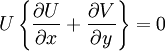
In addition, we have the two-dimensional mean continuity equation which reduces to:
|
| (4) |
Order of magnitude estimates
Now let's make an order of magnitude estimate for each of the terms. This procedure may seem trivial to some, or hopeless hand-waving to others. The fact is that if you fall either of these groups, you have missed something important. Learning to make good order-of-magnitude arguments and knowing when to use them (and when not to use them) are two of the most important skills in fluid mechanics, and especially turbulence. To do this right we will have to be very careful to make sure our estimates accurately characterize the terms we are making them for.
Naturally we should not expect changes of anything in the  - direction to scale the same as changes in the
  -direction, especially in view of the above. (This, after all, is the whole idea of "thin" shear flow.) So let's agree that we will pick a length scale, say
  , characteristic of changes or mean quantities in the -direction; i.e.
|
| (5) |

where for now ' ' means "of order of magnitude of". And we can do the same thing for changes of mean quantities in the -direction by defining a second lenght scale, say
  , to mean:
|
| (6) |

Note that both these scales will vary with the streamwise position where we evaluate them. A good choice for might be proportional to the local lateral extent of the flow (or its "width"), while is related to the distance from the source.
Consider the mean velocity in equation 10 in section "Wall-bounded turbulent flows". It occurs in five different terms:  alone; twice with -derivatives,
  and
and  ; and twice with -derivatives,
 and
and  . Now it would be tempting to simply pick a scale velocity for say
  , and use it to estimate all five terms, say as: ,
  ,
,  ,
,  , and
, and  . But this is much too naive, and fails to appreciate the true role of the terms we are evaluating.
Look at the examples shown in Figure ??. Our simple approach would provide an appropriate estimate for a jet if we took our velocity scale equal to the mean centerline velocity at a given streamwise location; i.e.,  . This is because both the mean velocity and the changes in the mean velocity across the flow are characterized by the centerline velocity. But by contrast, look at the wake. Even relatively close to the wake generator, the wake deficit,
 is small compared to the free stream velocity (i.e.
  ). So the obvious choice to scale
  is
is  On the other hand, an estimate for the velocity gradient across the flow of
  would be much too big, again because the deficit is so small. Obviously a better choice would be to use the centerline mean velocity deficit
  ; i.e.,
|
| (7) |

In the order of magnitude analysis below, we shall try to keep the discussion as general as possible by using  to characterize the mean velocity when it appears by itself, and
  to represent changes in the mean velocity. For the jet example of the preceding paragraph, both and are the same; i.e.
  and
and  . But for the wake they are different because of the external stream; i.e.,
  and
and  . If you can keep in mind why these differences exist among the various flows, it will be a lot easier to both understand the results and not confuse them.
Now we could distinguish changes of velocity in the -direction from those in the - direction. But this level of complexity is not necessary (at least for the examples considered here), especially since we have left the precise defenition of rather nebulous. What we can do is to use the same estimate for changes in the velocity as for the - direction, and define our length scale to make the estimate based on both correct; i.e.  . To see why this make sence physically and can be reasoned (as opposed to guessed), let's look at the wake. Pick a spot outside, near the edge of the wake fairly close the generator (say point A). Now proceed at constant far downstream in . Eventually the wake will have spread past you and you will be close enough to the centerline so the local mean velocity will be closer to
  than . Obviously we have simply traveled far enough at constant to ensure that is the proper scale for the changes in velocity in the - direction. If the distance downstream over which this change occured is taken as , then proper estimate is easily seen to be:
|
| (8) |

But this is exactly what we would have gotten by taking as we agreed above. We simply have absorbed any differences into our choice of . When considering specific problems and applying similarity techniques, the seemingly arbitrary choices here become quite precise constraints (as we shall see).
We still haven't talked about how to estimate the velocity scale for  , the cross-stream mean velocity component. From the continuity equation we know that:
|
| (9) |
From our considerations above, we know that:
|
| (10) |

If there is no mean cross flow in the external stream, then the scale for
is the same as the scale for changes in . Therefore,
|
| (11) |

It follows immediately that the order of magnitude of the cross-stream velocity is:
|
| (12) |

We might have expected something like this if we had thought about it. If the -velocity were of the same order as the - velocity, how could the flow in any sense be a "thin shear flow". On the other hand, it also makes sense that  since both are some measure of how the flow spreads/ Note that equation 12 would not be correct estimate for
  if there were an imposed cross-flow, since then we would have to consider and changes in separately (exactly as for ).
The mean pressure gradient term is always a problem to estimate at the outset. Therefore it is better to simply leave this problem alone, and see what is left at the end. In the estimates below you will see a question mark, which simply means we are postponing judgement until we have more information. Sometimes we will have to keep the term simply because we don't know enough to throw it away. Other times it will be obvious that it must remain because there is only one term left that must be balanced by something.
Now we have figured out how to estimate the order of magnitude of all the terms except the turbulence terms. For most problems this turns out to be pretty straight-forward if you remember our discussion of the pressure strain-rate terms. They so effectively distribute the energy that even that the three components of velocity are usually about the same order of magnitude. So if we choose a turbulence scale as simply  , then
  ,
,  ,
,  . But what about the Reynolds shear stress components like
  ? When acting against the mean shear to produce energy, they tend to be well-correlated and the maximum value of
  . Obviously the right choice though since some cross-stress like
  are identically zero in plane flows because of homogeniety. Allowing for the possibility of a Reynolds number dependent correlation coefficient will be sent to be especially important when the terms in the turbulence kinetic energy and dissipation equations are considered.
Streamwise momentum equation
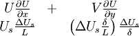
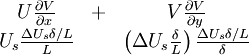
Let's look now at the -component of the mean momentum equation and write below each term its order of the magnitude.
|
|
|
|
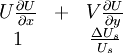
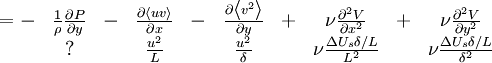
Now the survival of at least one of the terms on the left-hand side of the equation is the essence of free shear flow. Since the largest of these is the first, let's re-scale the others by deviding all the estimates by  . Now we have:
|
|
|
|
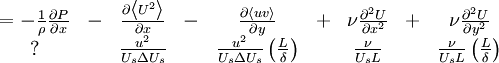
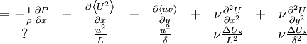
Just in case you need to be reminded, this is a turbulence course. Therefore almost all the interesting flows are at high Reynolds number. But what does this mean? Now we can say. It could mean the viscous terms in the mean momentum equation are negligible, which in tuurn means that:
|
|

and
|
|

Obviously the second criterion is much more stringent, since  is typically of order 10. When
 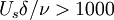 , the contributions of the viscous stresses are certainly negligible, at least as far as the -component of the mean mometum equation is concerned. But if
 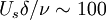 only, this is a pretty marginal assumption, and you might want to retain the last term in your analysis. Such is unfortunately the case in many experiments that are often at quite low Reynolds numbers.
So, what then, tou ask, do we do about the turbulence terms? To repeat this is a TURBULENCE course! Which means there is no way we are going to throw away all the turbulence terms on the right-hand side of the equation. There is no magic or hocus-pocus about this, you simply can't have turbulence without turbulence terms. And if there is no turbulence, we are really aren't too interested. So, what does this tell us? It tells us about ! Surprised? I bet you thought it would tell us about , right? Nope. Look at the right-hand side of the second equation of this subsection and the orders of magnitude below it. Almost always  ; sometimes much less and certainly no bigger. Then the biggest turbulence term is one involving the Reynolds shear stress
  which we have estimated as
 ![\left[ u^{2} / \left( U_{s} \Delta U_{s} \right) \right] \left( L / \delta \right)](/W/images/math/1/4/f/14f618b4914856b6ad60fb30e2fd8a55.png) . Hence there can be no turbulence terms at all unless:
. Hence there can be no turbulence terms at all unless:
|
|
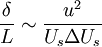
Wow! Look what we have learned about turbulence without ever solving a single equation. We know how the growth of our free shear flow relates to the turbulence intensity - at least in terms of order of magnitude. The simlarity theories described below will be able to actually deduce the - dependence of , again without solving the equations.
Does the argument above mean the other turbulence term is negligible since it is only of order  ? Well, no question it is usually small, typically less than 5%. But unlike the viscous terms, this term often does not get smaller the father we go in the streamwise direction. So the answer depends on the question we are asking and how accurately we want our answer to be. If we are asking only first order questions and are willing to accept errors in our solutions (or experiments) to within a 5-10 percent, then this normal stress is certainly negligible. Before you are ready to forget about this, consider the following: since
  typically, to first order free shear flows do not grow at all! So if you want to talk about whether
  for a particular shear flow is 0.095 instead of 0.09 (turbulence wars have been waged over less), then you better be dealing with a full desk - meaning these second order terms had better be retained in any calculation or experimental verification (like momentum or energy balances).
Much of the confusion in the literature about free shear flows comes from the failure to use second order accuracy to make second order statements. And even more unbelievably, most attempts to do so-called code validation of second-order turbulence models are based on mesurements which are only first order accurate. Now I know you think I am kidding - but try to do a simple momentum balance on the data to within order . Did I hear you say it was ridiculous to use second-order equations (like the Reynolds stress equations or even the kinetic energyequation) and determine constants to three decimal places using first order accurate data? Shhhh!!!! Your collegues might be annoyed unless you keeep this a secret.
Hopefully you have followed all this. If not, go forward and "faith" will come to you. I'll summarize how we do this:
- You have to look very carefully at the particular flow you wish to analyze.
- Then, based on physical reasoning and data (if you have it), you make estimates you think are appropriate.
- Then you use these estimates to decide which terms you have to keep, and which you can ignore.
- And when you are completely finished, you carefully look back to make sure that all the terms you kept really are important and remain important as the flow develops.
Finally, if you are really good at this, you look carefully to make sure that all the terms you kept do not all vanish at the same place (by going from positive to negative, for example). If this happens, then the terms you neglected may in fact be the only terms left in the equation thet are not exactly zero - oops! This can make fo some very interesting situations/ (The famous "critical layer" of boundary layer stability theory is an example of this.)
The transverse momentum equation
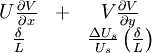
Now we must also cosider the transverse or -momentum equation. The most important thing we have to remember is that the - equation can NOT be considered indepedently from the -momentum equation. We would never consider trying to simplify a vector like  by dividing only one component by
  say to produce
  , since this would destroy the whole idea of a vector as having a direction. Similarly we must not do this for a vector equation. We have already decided thet the first term on the left-hand side of the -momentum equation was the term we had to keep, and we divided by its order of magnitude, , to make sure it was of order one. Thus we have already decided how we are going to scale all the components of the vector equation, and so we must do exactly the same thing here. but first we must estimate the order of magnitude of each term, exactly as before. Using our previous results, here's what we get:
|
|
|
|
Now dividing each term by , exactly as before, we obtain:
|
|
|
|
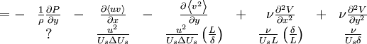
Unless you have seen this all before, the left-hand side is probably a surprise: none of the mean convection terms are of order one! In fact the only estimated term that is of order one in the whole equation is  and only because we have already agreed that
  had to be of order one to keep a turbulence term in the -momentum equation. Of course, there cannot be an equation with only a single term equal to zero, unless we have badly over-estimated its order of magnitude. Fortunately there is the pressure term left to balance it, so to first order in
  , the -momentum equation reduces to simply:
|
| (13) |
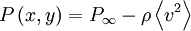
This simple equation has an equally simple interpretation. It says thet the change in the mean pressure is only due to the radisl gradient of the transverse component of the Reynolds normal stress,  .
.
We can integrate equation 13 across the shear layer from a given value of to infinity (or anywhere else for thet matter) to obtain:
|
| (14) |
If the free stream is at constant (or zero) mean velocity, then  , so we can write simply:
|
| (15) |
Either of these can be substituted into -momentum equation to eliminate the pressure entirely, as we shall show below.
Now since  typically
  , at least to first order in
  . Therefore one might be tempted to conclude that the small pressure changes across the flow are not important. And they are not, of course, if only the streamwise momentun is considered. But without this small mean pressure gradient across the flow, there would be no entrainment and no growth of the shear layer. In other words, the flow would remain parallel. clearly whether an effect is negligible or not depends on which question is being asked.
The free shear layer equations
If we assume the Reynolds number is always large enough that the viscous terms can be neglected, then as noted above, the pressure term in the terms of  and . Thus, to second-order in or
  , the momentum equations for a free shear flow reduce to a single equation:
|
| (14) |
![U \frac{\partial U}{ \partial x} + \left\{ V \frac{\partial U}{ \partial y} \right\} = - \frac{d P_{\infty}}{dx} - \frac{\partial }{ \partial y} \left\langle uv \right\rangle - \left\{ \frac{\partial }{ \partial x} \left[ \left\langle u^{2} \right\rangle - \left\langle v^{2} \right\rangle \right] \right\}](/W/images/math/8/0/3/80350420535045037d1488ad50b7b318.png)
As we have seen above, the second term on the left-hand side may or may not be important, depending on whether  or
or  . Clearly this depends on the velocity deficit (or excess) relative to the free stream. The term in brackets on the right-hand side is second-order (in
  ) compared to the others, and so could rigthgly be neglected. It has been retained for now since in some flows it does not vanish with increasing distance from the source. Moreover, it can be quite important when considering integrals of the momentum equation, since the profiles of
  and do not vanish as rapidly with increasing as do the other terms.
Two-dimensional Turbulent Jets
Turbulent jets are generated by a concentrated source of momentum issuing into an ambient environment. The state of the environment and the external boundary conditions are very important in determining how the turbulent flow evolves. The simplest case to consider is that in which the environment is at rest and unbounded, so all the boundary conditions are homogeneous. The jet itself can be assumed to isssue from a line source or a slot as shown in figure ??. The jet then evolves and spreads downstream by entraining mass from the surroundings which are at most in irrotational motion induced by the vortical fluid in the jet. But no new momentum is added to the flow, and it is this fact that distinguishes the jet from all other flows. As we shall see below the rate at which momentum crosses any - plane is not quite constant at the source value, however, due to the small streamwise pressure gradient arising from the turbulence normal stresses.
The avereged continuity equation can be integrated from the centerline (where it is zero by symmetry) to obtain , i.e.,
|
| (17) |
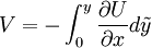
It immediately follows that the velocity at  is given by:
|
| (18) |
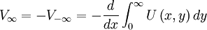
Twice the integral represents the total volume flow rate crossing a given - plane. Therefore it makes sense that the rate of increase of this integral is the enrainment velocity,  . Obviously, cannot be zero if the jet is to spread, at least in two-dimensional flow. It is easy to see that the entrainment velocity calculated from the integral is consistent with our order of magnitude estimate above (i.e.,
 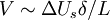 ). Note that the integral makes no sense if the mean velocity does not go to zero with increasing
  .
.
If the free stream is assumed to have zero streamwise velocity, then the scales for the velocity and gradienits of it are the same, so the equations reduce to simply equation 16 in the next section(need to edit) and the mean continuity equation. The latter can be multiplied by to yield:
|
| (19) |
When this is added to equation 16 from the next section(need to edit) the terms can be combined to obtain:
|
| (20) |
![\frac{\partial U^{2}}{\partial x} + \frac{\partial UV}{\partial y} + \frac{\partial \left\langle uv \right\rangle}{ \partial y} + \frac{ \partial }{ \partial x} \left[ \left\langle u^{2} \right\rangle - \left\langle v^{2} \right\rangle \right] = 0](/W/images/math/3/6/1/36118979922f6806a06471721247c648.png)
This can be integrated across the flow for any given value of to obtain:
|
| (21) |
![\frac{d}{dx} \int^{\infty}_{-\infty} \left[ U^{2} + \left( \left\langle u^{2} \right\rangle - \left\langle v^{2} \right\rangle \right) \right] dy = 0](/W/images/math/b/8/e/b8e1b299fd9f26e6e183f71ab5e6a375.png)
where we have assumed that , , and vanish as  . (Remember these assumptions the next time someone tries to tell you that a small co-flowing stream and modest background turbulence level in the external flow are not important.)
Equation (21) can in turn be integrated from the source, say  , to obtain:
|
| (22) |
![M_{o} = \int^{\infty}_{-\infty} \left[ U^{2} + \left( \left\langle u^{2} \right\rangle - \left\langle v^{2} \right\rangle \right) \right] dy](/W/images/math/4/7/7/4773ed7c55dc42800bed5b98bd9c59b3.png)
where  is the rate at which momentum per unit mass per unit length is added at the source. The first two terms of the itegral are the flux of streamwise momentum due to the mean flow and the turbulence. The last term is due to the streamwise pressure gradient obtained by integrating the -momentum equation.
This is a very powerful constraint, and together with the reduced governing equations allows determination of a similarity solution for this problem. Equation 22 also is of great value to experimentalists, since it can be used to confirm whether their measurements are valid and whether the flow indeed approximates a plane jet in an infinite environment at rest. Be fore-warned, most do not. And the explanations as to why range from hilarious to pathetic. Consider this, if you measure the velocity moments to within say 1%, then shouldn’t you be able to estimate the integral even more accurately, since the random errors from the integration should be reduced by one over the square root of the number of points you used in the integration? Be very wary of measurements which have not been tested against the momentum integral — for this and all flows. There is usually a reason the authors fail to mention it.
Similarity analysis of the plane jet
Foreword The results of this section are VERY MUCH at odds with those in all texts, including Pope 2000. There is an increasing body of literature to support the position taken, however, especially the multiplicity of solutions and the role of upstream or initial conditions. Since these ideas have a profound effect on how we think about turbulence, it is important that you consider both the old and the new, and be aware of why the conclusions are different.
The message you should take from the previous section is that regardless of how the plane jet begins, the momentum integral should be constant at . Note that Schneider (1985) has shown that the nature of the entrained flow in the neighborhood of the source can modify this value, especially for plane jets. Also the term  , while important for accounting for the momentum balance in the analysis below with no loss in generality.
The search for similarity solutions to the averaged equations of motion is exactly like the approach utilized in laminar flows (eg. Batchelor 1967) except that here there are more unknows than equations, i.e. the averaged equations are not closed. Thus solutions are sought which are of the form
|
| (23) |
|
| (24) |
|
| (25) |

where
|
| (26) |

The scale functions are functions of only, i.e.  and
and  only. Note that the point of departure from the traditional turbulence analyses was passed when it was not arbitrarily decided that
  , etc. (c.f. Tennekes and Lumley 1972, Townsend 1976, Pope 2000).
Now let you think there is something weird about the way we have written the form of the solutions we say we are looking for, consider this. Suppose you were looking for some - dependent quantities you could normalize the profiles by to make them all collepse together - like any experimentalist almost always does. Such a search is called the search for "scales" , meaning "scales" which collapse the data. Now precisely what does "collapse the data" really mean? Exactly this: "collapse the data" means that the form of the solution must be an -independent solution to the governing equations. But this is exactly what we are looking for in equations 23 and 24. Obviously we need to plug them into the averaged equations and see if such solution is possible. We already know which terms in these equations are important. What we want to do now is to see if these govering equations admit to solutions for which these terms remain important throughout the jet development. These are called equilibrium similarity solutions. Note that for any other form of solution, one or more terms could die off, so that others dominate.
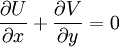
Differentiating equations 23 and 24 using the chain-rule, substituting into the averaged momentum equation, and clearing the terms yields:
|
| (27) |
![\left[ \frac{\delta}{U_{s}} \frac{ dU_{s}}{dx} \right] f^{2} - \left[ \frac{ \delta }{U_{s}} \frac{ dU_{s}}{dx} + \frac{d \delta}{dx} \right] f' \int^{\overline{y}}_{0} f\left( \overline{y}' \right) d \overline{y}' = \left[ \frac{R_{s}}{U^{2}_{s}} \right] g'](/W/images/math/1/3/8/1387f82704ef1ce41406b00e0964ee19.png)
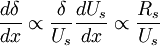
Now, all of the -dependence is in the square bracketed terms, so equilibrium similarity solutions are possible only if all the bracketed terms have the same -dependence, i.e.,
|
| (28) |
The coefficients of proportionality, say  and
and  respectively, can at most depend on the details of how the flow began; i.e., the mistery argument "*".
Substitution into the momentum integral yields to first order,
|
| (29) |

where
|
| (30) |
 and are parameters which also can at most depend on how the flow began (since every other dependence has been eliminated). Moreover, since is independent of , then
  and it follows that:
|
| (31) |
It's easy to see that all of the relations involving are proportional to , leaving only
|
| (32) |
![- \frac{1}{2} \left\{ f^{2} - f' \int^{\overline{y}}_{0} f \left( \overline{y}' \right) d \overline{y}' \right\} = \left[ \frac{R_{s}}{ U^{2}_{s} d \delta / d x} \right] g'](/W/images/math/5/5/d/55d8d32e51c1bf452fe8f00b98a3d067.png)
Thus the only remaining necessary condition for similarity is
|
| (33) |

Note that, unlike the similarity solutions encountered in laminar flows, it's possible to have a jet which is similar without having some form of power law behavior. In fact, the -dependence of the flow may not be known at all because of the closure problem. Nonetheless, the profiles will collapse with the local length scale. In fact, it is easy to show that the profiles for all plane jets will be alike, if normalized properly, even if the growth rates are quite different. The scale velocity can be defined to be the centerline velocity by absorbing an appropriate factor into the profile function  . Also, the entire factor in brackets on the right-hand side of equation 32 can be absorbed into the Reynolds stress profile,
  . Finally, if the length scale is chosen the same for all flows under consideration (e.g., the half-width, say
  , defined as the distance between the center and where
  ), then the similarity equation govering all jets reduces to,
|
| (34) |
where both  has been modified so that
  and
and  is just equal to
  with the factor
  absorbed into it. Thus all jets, regardless of initial conditions, will produce the same similarity velocity profile, when scaled with and . This will be not true for the Reynolds stress, however, unless the coefficient of proportionality between
  and
and  is the same for all plane jets. In general, it is not; so here is where the dependence on source conditions shows up.
It is immediately obvious from equation 32 that usual arbitrary choice of considerably restricts the possible solutions to those for which  , or plane jets which grow linearly. However, eben if the growth were linear under some conditions, there is nothing in the theory to this point which demands that the constant be universal and independent of how the jet began.
The idea that jets might all be described be the same asymptotic growth rate stems from the idea of a jet formed by a point source of momentum only, say  . Such a source must be infinitesimal in size, since any finite size will also provide a source of mass flow. In the absence of scaling parameters other than distance from the source, , the only possibilities are
  ,
,  ,
,  . Obviously , and the constants of proportionality can be assumed "universal" since there is only one way to create a point source jet, and this is also contarary to the usual assumption.
The problem with the point source idea is not in the idea itself, but that it has been accepted for so long by so many without justification as the asymptotic state of finite source jets. The usual line of argument (eg. Monin and Yaglom 1972) if one is presented at all is as follows. The jet entrains mass and the rate at which this occurs increases with distance downstream, so that the rate of mass entrainment ultimately overwhelms that added at the source. It is then inferred that the latter can be neglected. And what is the experimental proof for all this? Precisely that the profiles of  collapse to a single profile for all types of initial conditions. But as was demonstrated above, the mean momentum equation tells us that the mean velocity profiles will collapse to a single profile no matter what! If there is a dependence on the initial conditions it can only show up in the other turbulence moments, in profiles of the Reynolds shear stress normalized by
  (instead of ), and, of course, in itself. And guess what quantities no two experiments ever seem to agree on? — All of the above! Could all those experiments plus this nice theory with virtually no assumptions be wrong? Many think so. It is truly amazing how much good science people will throw away in order to hang-on to a couple of ideas that were never derived in the first place but assumed; namely, and the asymptotic independence of initial conditions. But then there are still many people who believe the world is flat.
George (1989) demonstrated for an axisymmetric jet that even simple dimensional analysis suggests that the classical theory is wrong, and the same arguments apply here. Suppose that in addition to momentum, mass is added at the source at a rate of  . Now there is an additional parameter to be considered, and as a consequence, an additional length scale given by
  . Thus the most that can be inferred from dimensional analysis is that
  ,
,  and
and  are functions of
  , with no insight offered into what the functions might be.
Implications of the Reynolds stress equations
George 1989 further argued that some insight into the growth rate of the jet can be obtained by considering the conditions for similarity solutions of the higher moment equations, in particular the kinetic energy equation. The choice of the kinetic energy equation for further analysis was unfortunate since it implicitly assumed that the three components of kinetic energy all scaled in the same manner. This is, in fact, true only if , which is certainly not true a priory for turbulent shear flows. Therefore, here the individual component equations of the Reynolds stress will be considered (as should have been done in George 1989).
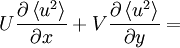
For the plane jet the equation for can be written to first oder (Tennekes and Lumley 1972) as
|
| (35) |
|
| (35) |
where  is the energy dissipation rate for .
By considering similarity forms for the new moments like
|
| (36) |
|
| (37) |
|
| (38) |
|
| (39) |
and using  , it's easy to show that similarity of the -equation is possible only if
|
| (40) |

|
| (41) |

|
| (42) |
|
| (43) |
All of these are somewhat surprising: The first (even though a second moment like the Reynolds stress) because the factor of is absent; the second, third and forth because it is present.
Similar equations can be written for the  ,
, , and
, and  -equations; i.e.
|
| (44) |
|
| (44) |
|
| (45) |
|
| (45) |
|
| (46) |
|
| (46) |
|
| (42) |

|
| (42) |
|
| (42) |
|
| (42) |
|
| (42) |
|
| (42) |
|
| (42) |