Introduction to turbulence/Wall bounded turbulent flows
From CFD-Wiki
| Nature of turbulence |
| Statistical analysis |
| Reynolds averaged equation |
| Turbulence kinetic energy |
| Stationarity and homogeneity |
| Homogeneous turbulence |
| Free turbulent shear flows |
| Wall bounded turbulent flows |
| Study questions
... template not finished yet! |
Contents |
Introduction
Without the presence of walls or surfaces, turbulence in the absence of density fluctuations could not exist. This is because it is only at surfaces that vorticity can actually be generated by an on-coming flow is suddenly brought to rest to satisfy the no-slip condition. The vorticity generated at the leading edge can then be diffused, transported and amplified. But it can only be generated at the wall, and then only at the leading edge at that. Once the vorticity has been generated, some flows go on to develop in the absence of walls, like the free shear flows we considered earlier. Other flows remained “attached” to the surface and evolve entirely under the influence of it. These are generally referred to as “wall-bounded flows” or “boundary layer flows”. The most obvious causes for the effects of the wall on the flow arise from the wall-boundary conditions. In particular,
- The kinematic boundary condition demands that the normal velocity of
the fluid on the surface be equal to the normal velocity of the surface. This means there can be no-flow through the surface. Since the velocity normal to the surface cannot just suddenly vanish, the kinematic boundary condition ensures that the normal velocity components in wall-bounded flows are usually much less than in free shear flows. Thus the presence of the wall reduces the entrainment rate. Note that viscosity is not necessary in the equations to satisfy this condition, and it can be met even by solutions to to the inviscid Euler’s equations.
- The no-slip boundary condition demands that the velocity component tangential to the wall be the same as the tangential velocity of the wall. If the
wall is at rest relative, then the no-slip condition demands the tangential flow velocity be identically zero at the surface.
Figure 8.1: Flow around a simple airfoil without separation.
It is the no-slip condition, of course, that led Ludwig Prandtl1 to the whole
idea of a boundary layer in the first place. Professor Prandt literally saved fluid mechanics from d’Alembert’s paradox: the fact that there seemed to be no drag in an inviscid fluid (not counting form drag). Prior to Prandtl, everyone thought that as the Reynolds number increased, the flow should behave more and more like an inviscid fluid. But when there were surfaces, it clearly didn’t. Instead of behaving like those nice potential flow solutions (like around cylinders, for example), the flow not only produced drag, but often separated and produced wakes and other free shear flows. Clearly something was very wrong, and as a result fluid mechanics didn’t get much respect from engineers in the 19th century.
And with good reason: how useful could a bunch of equations be if they couldn’t
find viscous drag, much less predict how much. But Prandtl’s idea of the boundary
layer saved everything.
Prandtl’s great idea was the recognition that the viscous no-slip condition could not be met without somehow retaining at least one viscous stress term in the equations. As we shall see below, this implies that there must be at least two length scales in the flow, unlike the free shear flows we considered in the previous chapter for which the mean flow could be characterized by only a single length scale. The second length scale characterizes changes normal to the wall, and make it clear precisely which viscous term in the instantaneous equations is important.
Review of laminar boundary layers
Let’s work this all out for ourselves by considering what happens if we try to
apply the kinematic and no-slip boundary conditions to obtain solutions of the
Navier-Stokes equations in the infinite Reynolds number limit. Let’s restrict our
attention for the moment to the laminar flow of a uniform stream of speed,  ,
around a body of characteristic dimension, D, as shown in Figure 8.1. It is easy
to see the problem if we non-dimensionalize our equations using the free stream
boundary condition and body dimension. The result is:
,
around a body of characteristic dimension, D, as shown in Figure 8.1. It is easy
to see the problem if we non-dimensionalize our equations using the free stream
boundary condition and body dimension. The result is:
|
| (1) |
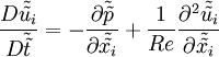
where  ,
,  ,
,  and
and 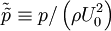 . The kinematic viscosity,
  has disappeared entirely, and is included in the Reynolds number defined by:
|
| (2) |

Now consider what happens as the Reynolds number increases, due to the increase of  or
or  , or even a decrease in the viscosity. Obviously the viscous terms become relatively less important. In fact, if the Reynolds number is large enough it is hard to see at first glance why any viscous term should be retained at all. Certainly in the limit as
  , our equations must reduce to Euler’s equations which have no viscous terms at all; i.e., in dimensionless form,
|
| (3) |
Now if we replace the Navier-Stokes equations by Euler’s equations, this presents no problem at all in satisfying the kinematic boundary condition on the body’s surface. We simply solve for the inviscid flow by replacing the boundary of the body by a streamline. This automatically satisfies the kinematic boundary condition. If the flow can be assumed irrotational, then the problem reduces to a solution of Laplace’s equation, and powerful potential flow methods can be used.
In fact, for potential flow, it is possible to show that the flow is entirely determined by the normal velocity at the surface. And this is, of course, the source of our problem. There is no role left for the viscous no-slip boundary condition. And indeed, the potential flow has a tangential velocity along the surface streamline that is not zero. The problem, of course, is the absence of viscous terms in the Euler equations we used. Without viscous stresses acting near the wall to retard the flow, the solution cannot adjust itself to zero velocity at the wall. But how can viscosity enter the equations when our order-of-magnitude analysis says they are negligible at large Reynolds number, and exactly zero in the infinite Reynolds number limit. At the end of the nineteenth century, this was arguably the most serious problem confronting fluid mechanics.
Prandtl was the first to realize that there must be at least one viscous term
in the problem to satisfy the no-slip condition. Therefore he postulated that the
strain rate very near the surface would become as large as necessary to compensate for the vanishing effect of viscosity, so that at least one viscous term remained. This very thin region near the wall became known as Prandtl’s boundary layer, and the length scale characterizing the necessary gradient in velocity became known as the boundary layer “thickness”.
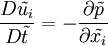
Prandtl’s argument for a laminar boundary layer can be quickly summarized using the same kind of order-of-magnitude analysis we used in Chapter 7 (here necessary make navigation !!!). For the leading viscous term:
|
| (4) |
where  is the new length scale characterizing changes normal to the plate near the wall and we have assumed
  . In fact, for a boundary layer next to walls driven by an external stream speed
  . For the leading convection term:
|
| (5) |

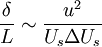
The viscous term can survive only if it is the same order of magnitude as the convection term. Hence it follows that we must have:
|
| (6) |

This in turn requires that new length scale must satisfy:
|
| (7) |
![\delta \sim \left[ \frac{\nu L}{U_{s}} \right]^{1/2}](/W/images/math/d/c/d/dcd40e1c6fe0b947b08a89273c8922a6.png)
or
|
| (8) |
![\frac{\delta}{L} \sim \left[ \frac{\nu }{U_{s} L} \right]^{1/2}](/W/images/math/5/1/0/5109f2a3964f3b5997eeeee387ad7f8c.png)
Thus, for a laminar flow grows like  . Now if you go back to your fluid mechanics texts and look at the similarity solution for a Blasius boundary layer, you will see this is exactly right if you take
  , which is what we might have guessed anyway.
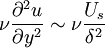
It is very important to remember that the momentum equation is a vector equation, and we therefore have to scale all components of this vector equation the same way to preserve its direction. Therefore we must carry out the same kind of estimates for the cross-stream momentum equations as well. For a laminar boundary layer this can be easily be shown to reduce to:
|
| (9) |
![\left[ \frac{\delta}{L} \right] \left\{ \frac{ \partial \tilde{\tilde{ u}}}{ \partial \tilde{\tilde{t}}} + \tilde{\tilde{u}} \frac{\partial \tilde{\tilde{ u}} }{\tilde{\tilde{ x}}}+ \tilde{\tilde{v}} \frac{\partial \tilde{\tilde{ v}} }{\tilde{\tilde{ y}}} \right\} = - \frac{ \partial \tilde{\tilde{p}}_{\infty}}{ \partial \tilde{\tilde{ y}} } + \frac{1}{Re} \left[ \frac{\delta}{L} \right] \left\{ \frac{ \partial^{2} \tilde{\tilde{v}} }{ \partial \tilde{\tilde{ y}}^{2}} \right\} + \frac{1}{Re} \left\{ \frac{ \partial^{2} \tilde{\tilde{v}} }{ \partial \tilde{\tilde{ x}}^{2}} \right\}](/W/images/math/1/d/8/1d809934e9ae0d115665576eb95a0b1c.png)
Note that a only single term survives in the limit as the Reynolds number goes to
infinity, the cross-stream pressure gradient. Hence, for very large Reynolds number, the pressure gradient across the boundary layer equation is very small. Thus the pressure in the boundary is imposed on it by the flow outside the boundary layer. And this flow outside the boundary layer is governed to first order by Euler’s equation.
The fact that the pressure is imposed on the boundary layer provides us an
easy way to calculate such a flow. First calculate the inviscid flow along the
surface using Euler’s equation. Then use the pressure along the surface from this inviscid solution together with the boundary layer equation to calculate the boundary layer flow. If you wish, you can even use an iterative procedure where you recalculate the outside flow over a streamline which was been displaced from the body by the boundary layer displacement thickness, and then re-calculate the boundary layer, etc. Before modern computers, this was the only way to calculate the flow around an airfoil, for example.
The "outer" turbulent boundary layer
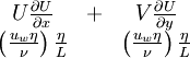
The understanding of turbulent boundary layers begins with exactly the same averaged equations we used for the free shear layers of Chapter 7(here necessary to add link!!!); namely,
 -component:
|
| (10) |

 -component:
|
| (11) |

two-dimensional mean continuity
|
| (12) |
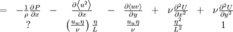
In fact, the order of magnitude analysis of the terms in this equation proceeds exactly the same as for free shear flows. If we take  , then the ultimate problem again reduces to how to keep a turbulence term. And, as before this requires:
|
| (00) |
No problem, you say, we expected this. But the problem is that by requiring this be true, we also end up concluding that even the leading viscous term is also negligible! Recall that the leading viscous term is of order:
|
| (13) |

compared to the unity.
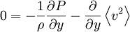
In fact to leading order, there are no viscous terms in either component of the
momentum equation. In the limit as  , they are exactly the same as for the free shear flows we considered earlier; namely,
|
| (14) |
and
|
| (15) |
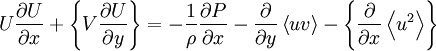
And like the free shear flows these can be integrated from the free stream to a
given value of to obtain a single equation:
|
| (16) |
![U \frac{\partial U}{ \partial x} + V \frac{\partial U}{ \partial y} = - \frac{d P_{\infty}}{dx} - \frac{\partial }{ \partial y} \left\langle uv \right\rangle - \left\{ \frac{\partial}{\partial x} \left[ \left\langle u^{2} \right\rangle - \left\langle v^{2} \right\rangle \right] \right\}](/W/images/math/3/d/d/3ddd8fc067d2b2c5ee66fc50ba0343fc.png)
The last term in brackets is the gradient of the difference in the normal Reynolds stresses, and is of order  compared to the others, so is usually just ignored. The bottom line here is that even though we have attempted to carry out an order of magnitude analysis for a boundary layer, we have ended up with exactly the equations for a free shear layer. Only the boundary conditions are different— most notably the kinematic and no-slip conditions at the wall. Obviously, even though we have equations that describe a turbulent boundary layer, we cannot satisfy the no-slip condition without a viscous term. In other words, we are right back where we were before Prandtl invented the boundary layer for laminar flow! We need a boundary layer within the boundary layer to satisfy the no-slip condition. In the next section we shall in fact show that such an inner boundary layer exists. And that everything we analysed in this section applies only to the outer boundary layer — which is NOT to be confused with the outer flow which is non-turbulent and still governed by Euler’s equation. Note that the presence of
  in our outer boundary equations means that (to first order in the turbulence intensity), the pressure is still imposed on the boundary layer by the flow outside it, exactly as for laminar boundary layers (and all free shear flows, for that matter).
The “inner” turbulent boundary layer
We know that we cannot satisfy the no-slip condition unless we can figure out
how to keep a viscous term in the governing equations. And we know there can
be such a term only if the mean velocity near the wall changes rapidly enough so
that it remains, no matter how small the viscosity becomes. In other words, we
need a length scale for changes in the -direction very near the wall which enables us keep a viscous term in our equations. This new length scale, let’s call it  , is going to be much smaller than , the boundary layer thickness. But how much smaller?
Obviously we need to go back and look at the full equations again, and re-scale
them for the near wall region. To do this, we need to first decide how the mean
and turbulence velocities scale near the wall scale. We are clearly so close to the wall and the velocity has dropped so much (because of the no-slip condition) that it makes no sense to characterize anything by . But we don’t have anyway of knowing yet what this scale should be, so let’s just call it  and define it later. Also, we do know from experiment that the turbulence intensity near the wall is relatively high (30% or more). So there is no point in distinguishing between a turbulence scale and the mean velocity, we can just use for both. Finally we will still use to characterize changes in the -direction, since these will vary no more rapidly than in the outer boundary layer above this very near wall region we are interested in.
For the complete -momentum equation we estimate
|
| (00) |
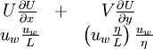
|
| (00) |
where we have used the continuity equation to estimate  near the wall.
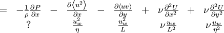
Now as always, we have to decide which terms we have to keep so we know what to compare the others with. But that is easy here, we MUST insist that at least one viscous term survive. Since the largest is of order  , we can divide by it to obtain:
|
| (00) |
|
| (00) |
Now we have an interesting problem. We have the power to whether the Reynolds shear stress term survives or not by our choice of ; i.e. we can pick  or
or  . Note that we can not choose it so this term blows up, or else our viscous term will not be at least equal to the leading term. The most general choice is to pick
  so the Reynolds shear stress remains too. (This is called the distinguished limit in asymptotic analysis.) By making this choice we eliminate the necessity of having to go back and find there is another layer in which only the Reynolds stress survives — as we shall see below. Obviously if we choose , then all the other terms vanish, except for the viscous one. In fact, if we apply the same kind of analysis to the -mean momentum equation, we can show that the pressure in our near wall layer is also imposed from the outside. Moreover, even the streamwise pressure gradient disappears in the limit as
 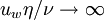 . These are relatively easy to show and left as exercises.
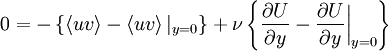
So to first order in 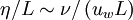 , our mean momentum equation for the near wall region reduces to:
|
| (17) |
![0 \approx \frac{\partial}{\partial y} \left[ - \left\langle uv \right\rangle + \nu \frac{\partial U}{ \partial y} \right]](/W/images/math/4/9/8/4988d861e7738f9b1f65330d845e58ca.png)
In fact, this equation is exact in the limit as  , but only for the very near wall region!
Equation (17) can be integrated from the wall to location to obtain:
|
| (18) |
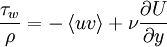
From the kinematic and no-slip boundary conditions at the wall we immediately know that  . We also know that the wall shear stress is given by:
|
| (19) |
Substituting this we obtain our equation for the very near wall (in the limit of
infinite Reynolds number) as:
|
| (20) |
We immediately recognize one of the most important ideas in the history of boundary layer theory; namely that in the limit of infinite Reynolds number the total stress in the wall layer is constant. Not surprisingly, the wall layer is referred to quite properly as the Constant Stress Layer. It is important not to forget (as many who work in this field do) that this result is valid only in the limit of infinite Reynolds number. At finite Reynolds numbers the total stress is almost constant, but never quite so because of the terms we have neglected. This difference may seem slight, but it can make all the difference in the world if you are trying to build an asymptotically correct theory, or even just understand your experiments.
Before leaving this section we need to resolve the important questions of what
is , our inner velocity scale. It is customary to define something called the friction velocity, usually denoted as  , by:
, by:
|
| (21) |

Now using this, equation 20 can be rewritten as:
|
| (22) |
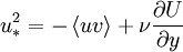
It should be immediately obvious that the choice is  ; in other words, the friction velocity is the appropriate scale velocity for the wall region. It follows immediately from our considerations above that the inner length scale is
  .
.
An interesting consequence of these choices is that the inner Reynolds number is
unity; i.e.  , meaning that viscous and inertial terms are about the same. But then this is precisely why we defined as we did in the first place — to ensure that viscosity was important.
It is important not to read too much into the appearance of the wall shear stress in our scale velocity. In particular, it is wrong to think that it is the shear stress that determines the boundary layer. In fact, it is just the opposite: the outer boundary layer determines the shear stress. If you have trouble seeing this, just turn off the outer flow and the boundary layer disappears. The wall shear stress appears in the scale velocity only because of the constant stress layer which changes the Reynolds stress imposed by the outer flow into the viscous stress on the wall.
Finally we can use our new length scale to define where we are in this near
wall layer. In fact, we can introduce a whole new dimensionless coordinate called
 defined as:
|
| (23) |
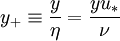
When moments of the velocity field, for example, are normalized by (to the appropriate power) and plotted as functions of , they are said to be plotted in “inner” variables. Similarly, we can non-dimensionalize equation 20 using inner variables and rewrite it as simply:
|
| (24) |
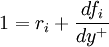
where if we suppress for the moment a possible -dependence we can write:
|
| (25) |
and
|
| (26) |
By contrast an “outer” dimensionless coordinate,  , is defined by:
|
| (27) |

In terms of these coordinates the outer equations (for the mean flow) are generally considered valid outside of  or so. And the inner equations are needed inside of
  if we take
  .
.  is defined to be equal to the value of y at which the mean velocity in the boundary layer is 0.99% of its free stream value, .
It is easy to see that the ratio of to is the local Reynolds number  where
where
|
| (28) |

(8.28)
Obviously the higher the value of , the closer the inner layer will be to the wall relative to . On the other hand, since the wall friction (and hence ) drops with increasing distance downstream, both the outer boundary layer and inner boundary grow in physical variables (i.e., the value of y marking their outer edge increases). Sorting all these things out can be very confusing, so it is very important to keep straight whether you are talking about inner, outer or physical variables.
The viscous sublayer
The linear sublayer
It should be clear from the above that the viscous stress and Reynolds stress
cannot both be important all the way across the constant stress layer. In fact,
inside  , the Reynolds stress term is negligible (to within a few percent), so very near the wall equation 20 reduces to:
|
| (29) |

or in inner variables:
|
| (30) |

This equation is exact right at the wall, for any Reynolds number. It can immediately be integrated to obtain the leading term in an expansion of the velocity about the wall as:
|
| (31) |
or in physical variables
|
| (32) |
Note that some authors consider the extent of the linear sublayer to be  , but by the Reynolds stress has already begun to evolve, making the approximations above invalid. Or said another way, the linear approximation is only good to within about 10% at ; and the linear approximation deteriorates rapidly outside this.
This linear region in the mean velocity at the wall is one of the very few EXACT
solutions in all of turbulence. There are NO adjustable constants! Obviously
it can be used with great advantage as a boundary condition in numerical solutions — if the resolution is enough to resolve this part of the flow at all. And it has great advantages for experimentalists too. They need only resolve the velocity to to be able to get an excellent estimate of the wall shear stress.
Unfortunately, few experiments can resolve this region. And unbelievably, even some who do choose to ignore the necessity of satisfying equation 8.31 or 8.32. Look at it this way, if these equations are not satisfied by the data, then either the Navier-Stokes equations are wrong, or the data is wrong. If you think the former and can prove it, you might win a Nobel prize.
It should be obvious why this subregion very near the wall is usually referred
to as the linear sublayer. It should not be confused with the term viscous sublayer, which extends until the mean flow is dominated by the Reynolds stress alone at about .
The important point is that the mean velocity profile is linear at the wall! It
is easy to show using the continuity equation and the wall boundary conditions
on the instantaneous velocity at the wall that the Reynolds stress is cubic at the wall; i.e., 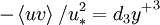 . See if you can now use equation 8.20 to show that this implies that a fourth order expansion of the mean velocity at the wall yields:
|
| (33) |
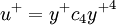
where  . It is not clear at this point whether c4 (and d3) are Reynolds number dependent or not. Probably not, but they are usually taken as constant anyway by turbulence modelers seeking easy boundary conditions. Note that this fourth order expansion is a good description of the mean velocity only out to
  , beyond which the cubic expansion of the Reynolds stress (on which it is based) starts to be invalid.
The sublayers of the constant stress region
As we move out of the linear region very close to the wall the Reynolds stress
rapidly develops until it overwhelms the viscous stress. Also, as we move outward, the mean velocity gradient slowly drops until the viscous stress is negligible compared to the Reynolds shear stress. In fact, by , the viscous shear stress is less than a percent or so of the Reynolds shear stress.
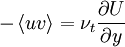
Thus outside this point we have only:
|
| (34) |

In other words, the Reynolds shear stress is itself nearly constant. Viscous effects on the mean flow are gone, and only the inertial terms from the fluctuating motion remain. This region is referred to as the inertial sublayer.
Figure 8.2 summarizes the important regions of a turbulent boundary layer.
The constant stress layer has two parts: a viscous sublayer and an inertial sublayer. The viscous sublayer itself has two identifiable regions: the linear sublayer where only viscous shear stresses are important, and a buffer layer in which both viscous and Reynolds shear stresses are important. And as we shall see later, some (me among them) believe that the lower part of the inertial sublayer ( approximately) is really a mesolayer in which the Reynolds shear stress is constant at
  , but the energetics of the turbulence (the multi-point equations) are still influenced by viscosity. Or said another way, the mean flow equations are indeed inviscid, but the multi-point equations for the turbulence are not. This close to the wall, there simply is not the scale separation between the energy and dissipative scales required for them to be.
The inertial sublayer
The inertial sublayer is one of the most discussed and debated subjects in Fluid Mechanics. There is one whole school of thought that says the mean profile is logarithmic — quite independent of whether the external flow is a boundary layer, a pipe, a channel, or for that matter about anything you can think of. Moreover, it is usually argued that the three parameters in this universal log profile are themselves universal constants.
This whole idea of a universal log law has pretty much been elevated to the
level of the religion — and why not? Life becomes a lot simpler if some things can be taken as known to be true. And even the word, universality has a nice ring to it. For example, some go so far as to say that we can be so sure of these things that we don’t even need to bother measure down below the “log” layer, since we already know the answer — we need only find the ‘shear stress’ which fits the universal log profile onto our data, and that’s the shear stress. And if the measurements down in the linear region don’t collapse when plotted as  versus
  and the inferred value of , why then clearly the measurements of U or y must be wrong down there. The possibility that the log law might be wrong, or even that the parameters might not be constant is just too painful to contemplate.

Figure 2.
Sketch showing the various regions of the turbulent boundary layer in inner and outer variables. Note that in is less than approximately 3000, then the inertial layer cannot be present, and for less than about 300, the mesolayers extend into the outer layer.
So no matter how much evidence piles up to the contrary, the universalists persist in their “beliefs” – a lot like the people who still believe that the earth is flat (There really are people who still believe the earth is flat, and they even have ‘explanations’ for all our observations that suggest it is not. Turbulence ‘experts’ are capable of these kinds of arguments too). It just makes the earth so much easier to draw.
Now you probably suspect from the tone of the above that I am not a member of the universalist school. And you are certainly right — and I don’t believe the earth is flat either. But I am not one of the ‘other’ group either — the so-called power-law school who believe that the mean velocity profile in this region is given by a power law. The ‘power law people’ are at somewhat of a disadvantage since their parameters are Reynolds number dependent. The fact that their power laws may fit the data better is scoffed at, of course, by the universalists who naturally believe any data for which their universal log law does not fit perfectly must be wrong, or certainly in need of careful manipulation.
So where to these ideas come from? And why do people hold them so zealously? Well, the first is easy and we shall see below. The answer to the second question is probably the same as for every religious quarrel that has ever been — the less indisputable evidence there is for an idea, the more people argue that there is.
So back to question one. Here in a nutshell is the answer: Let’s consider a very simple closure solution to this problem in only the inertial sublayer, say an eddy viscosity; i.e.,
|
| (35) |
Now let’s plug this into our momentum equation to obtain:
|
| (36) |

Obviously if we can think of a good form for the eddy viscosity,  , we can integrate this to find the mean velocity profile, U.
Consider the following:
- We are in a flow region where the viscous stress is negligible.
- The only parameters we have to work with are the distance from the wall,
, and the friction velocity, .
It follows immediately on dimensional grounds alone that:
|
| (37) |
![\nu_{t} = C u_{*} \left[ y + a \right]](/W/images/math/2/e/2/2e2a742f95abcc41cea26bf39f57c549.png)
where the coefficient  must be exactly constant in the limit of infinite Reynolds number as must the additive “offset”
  . Note that an offset is necessary since we really don’t have any idea how big an eddy is relative to the wall, nor what the effect of the viscous sublayer beneath us is.
Now here’s the problem: What do we mean by infinite Reynolds number — which is of course the only limit in which our inner equations are valid anyway?
For a parallel flow like a pipe or channel where all the -derivatives of mean quantities are zero (i.e., homogeneous in ) , this is no problem. But for a developing flow like a boundary layer or wall jet it is a BIG problem since the further you go, the bigger the Reynolds number gets, so you never stop evolving. Let’s treat these two cases separately.
For the flows homogeneous in x, we can take C(Re) and a = a(Re) to be Reynolds number dependent, but independent of y. This implies we can integrate equation 8.36 using equation 8.37 to obtain:
homogeneous flows
|
| (38) |
![u^{+} = C_{i} \left( Re \right) ln \left[ y^{+} a \left( Re \right)^{+} \right] + B_{i} \left( Re \right)](/W/images/math/5/2/6/526886dd83fc69425960e4a2c01e0c89.png)
where B(Re) is the integration constant. Since in the limit of infinite Reynolds number, our original momentum equation was independent of Reynolds number, then so must our solution be in the same limit; i.e.
|
| (39) |
|
| (40) |
|
| (41) |
This is, of course, the usual log law – but with an offset. And  is the inverse of the usual von Karman “constant”.
Now what happens in a developing boundary layer. Many people assume
nothing different. But then the whole idea of a boundary layer is that it spreads, so it is the departures from a parallel flow that make it a boundary layer in the first place. The most obvious way (maybe the only way) to account for the variation of the local Reynolds number as the flow develops is to include a factor  in our eddy viscosity; i.e.,
|
| (42) |
where  itself is probably very small, depends on Reynolds number, and must be asymptotically constant. Since we know the flow very near the wall is almost parallel, it is obvious that is going to be have to be quite small. But it is easy to show that no matter how small is, unless it is identically zero, our equation will never integrate to a logarithm.
In fact, we obtain:
|
| (43) |
![u^{+} = C_{i} \left( Re \right) \left[ y^{+} + a^{+} \right]^{\alpha} + B_{i} \left( Re \right)](/W/images/math/8/f/1/8f18063b245ef7b1159c985bb76c26df.png)
where as before all the parameters must be asymptotically constant. As you can
see this is a power law.
On the other hand, suppose the flow is exactly parallel, like a channel or a
pipe. Then our would be exactly zero, and we get a logarithmic profile. This is to me one of the great mysteries of calculus: how a tiny infinitesimal can change a logarithm to a power law.
In fact, other arguments based on functional analysis and quite independent of closure models can produce the same results, and show that the additive parameter for the power law is identically zero. Moreover, it is possible using a powerful new method call Near-asymptotics to actually deduce the Reynolds number dependence of most of the parameters in both the log and the power laws. This is an area undergoing great development at the moment. My advice is: Reject any simple argument which dismisses these new developments. They may not be as simple as the old log law, but they might have the advantage of being right.