From CFD-Wiki
Instantaneous equations
The instantaneous continuity equation (1), momentum equation (2) and energy equation (3) for a compressible fluid can be written as:
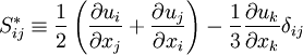
For a Newtonian fluid, assuming Stokes Law for mono-atomic gases, the viscous stress is given by:

| (4) |
Where the trace-less viscous strain-rate is defined by:
| (5) |
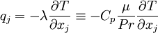
The heat-flux,  , is given by Fourier's law:
| (6) |
Where the laminar Prandtl number  is defined by:

| (7) |
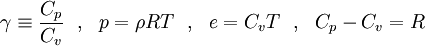
To close these equations it is also necessary to specify an equation of state. Assuming a calorically perfect gas the following relations are valid:
| (8) |
Where  ,
,  ,
,  and
and  are constant.
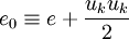
The total energy  is defined by:
| (9) |
Note that the corresponding expression (15) for Favre averaged turbulent flows contains an extra term related to the turbulent energy.
Equations (1)-(9), supplemented with gas data for , ,  and perhaps , form a closed set of partial differential equations, and need only be complemented with boundary conditions.
Favre averaged equations
It is not possible to solve the instantaneous equations directly for most engineering applications. At the Reynolds numbers typically present in real cases these equations have very chaotic turbulent solutions, and it is necessary to model the influence of the smallest scales. Most turbulence models are based on one-point averaging of the instantaneous equations. The averaging procedure will be described in the following sections.
Averaging
Let  be any dependent variable. It is convenient to define
two different types of averaging of :
be any dependent variable. It is convenient to define
two different types of averaging of :
|
(10) |

|

| (11) |

|
Note that with the above definitions  , but
, but  .
.
Open turbulent equations
In order to obtain an averaged form of the governing equations, the instantaneous continuity equation (1), momentum
equation (2) and energy equation (3) are time-averaged. Introducing a density weighted time average decomposition (11) of  and , and a standard time average decomposition (10) of
  and
and  gives the following exact open equations:
![\frac{\partial \overline{\rho}}{\partial t} +
\frac{\partial}{\partial x_i}\left[ \overline{\rho} \widetilde{u_i} \right] = 0](/W/images/math/d/c/d/dcd521718edfb790fcf5915dfff51dde.png)
| (12) |
![\frac{\partial}{\partial t}\left( \overline{\rho} \widetilde{u_i} \right) +
\frac{\partial}{\partial x_j}
\left[
\overline{\rho} \widetilde{u_i} \widetilde{u_j} + \overline{p} \delta_{ij} +
\overline{\rho u''_i u''_j} - \overline{\tau_{ji}}
\right]
= 0](/W/images/math/8/b/6/8b6ccd8ae759989435f91b921c8f73b1.png)
| (13) |
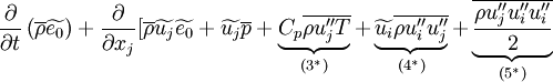
![\frac{\partial}{\partial t}\left( \overline{\rho} \widetilde{e_0} \right) +
\frac{\partial}{\partial x_j}
\left[
\overline{\rho} \widetilde{u_j} \widetilde{e_0} +
\widetilde{u_j} \overline{p} + \overline{u''_j p} +
\overline{\rho u''_j e''_0} + \overline{q_j} - \overline{u_i \tau_{ij}}
\right]
= 0](/W/images/math/1/e/5/1e51a93eafbd4986d688c8b17b5cb4dd.png)
| (14) |
The density averaged total energy  is given by:
| (15) |
Where the turbulent energy,  , is defined by:

| (16) |
Equation (12), (13) and (14) are referred to as the Favre averaged Navier-Stokes equations.  ,
,  and are the primary solution variables. Note that this is an open set of partial differential equations that contains several unkown correlation terms. In order to obtain a closed form of equations that can be solver it is neccessary to model these unknown correlation terms.
Approximations and modeling
To analyze equation (12), (13) and (14) it is convenient to rewrite the unknown terms in the following way:
| (17) |
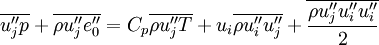
| (18) |
| (19) |
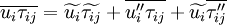
| (20) |
Where the perfect gas relations (8) and Fourier's law (6) have been used. Note also that fluctuations in the molecular viscosity, , have been neglected.
Inserting (17)-(20) into (12), (13) and (14) gives:
-
| (21) |
![\frac{\partial}{\partial t}\left( \overline{\rho} \widetilde{u_i} \right) +
\frac{\partial}{\partial x_j}
\left[
\overline{\rho} \widetilde{u_i} \widetilde{u_j} + \overline{p} \delta_{ij} +
\underbrace{\overline{\rho u''_i u''_j}}_{(1^*)} - \widetilde{\tau_{ji}} -
\underbrace{\overline{\tau''_{ji}}}_{(2^*)}
\right]
= 0](/W/images/math/0/c/1/0c1b4f5f40696025d26ab8a4f9aab2ab.png)
| (22) |
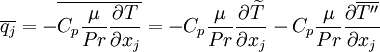
|
![- C_p \frac{\mu}{Pr} \frac{\partial \widetilde{T}}{\partial x_j}
- \underbrace{C_p \frac{\mu}{Pr} \frac{\partial \overline{T''}}
{\partial x_j}}_{(6^*)}-
\widetilde{u_i} \widetilde{\tau_{ij}} -
\underbrace{\overline{u''_i \tau_{ij}}}_{(7^*)} -
\underbrace{\widetilde{u_i} \overline{\tau''_{ij}}}_{(8^*)}
]
= 0](/W/images/math/d/d/0/dd02145b9c12b0593a92b6111faf8b17.png)
| (23) |
The terms marked with  are unknown, and have to be modeled in some way.
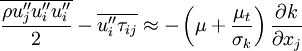
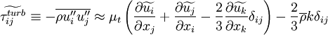
Term  and
and  can be modeled using an eddy-viscosity assumption for the Reynolds stresses,
  :
:
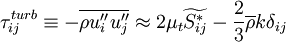
| (24) |
Where  is a turbulent viscosity, which is estimated with a turbulence model. The last term is included in order to ensure that the trace of the Reynolds stress tensor is equal to
  , as it should be.
Term  and
and  can be neglected if:
| (25) |
This is true for virtually all flows.
Term  , corresponding to turbulent transport of heat, can be modeled using a gradient approximation for the turbulent heat-flux:
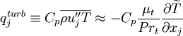
| (26) |
Where  is a turbulent Prandtl number. Often a constant
  is used.
Term  and
and  , corresponding to turbulent transport and molecular diffusion of turbulent energy, can be neglected if the turbulent energy is small compared to the enthalpy:
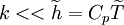
| (27) |
This is a reasonable approximation for most flows below the hyper-sonic regime. A better approximation might be a gradient expression of the form:
| (28) |
Where  is a model constant. This approximation will not be included in the derived formulas below. Instead term and will be set to zero in the energy equation.
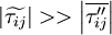
Term  is an artifact from the Favre averaging. It is related to heat conduction effects associated with temperature fluctuations.It can be be neglected if:
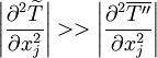
| (29) |
This is true for virtually all flows, and has been assumed in all follwing equations.
Closed approximated equations
To summarize, the governing equations (21)-(23), with assumptions (24), (25), (26), (27) and (29) can be written as in (30)-(39). These equations are valid for a perfect gas. Note also that all fluctuations in the molecular viscosity have been neglected.
-
| (30) |
![\frac{\partial}{\partial t}\left( \overline{\rho} \widetilde{u_i} \right) +
\frac{\partial}{\partial x_j}
\left[
\overline{\rho} \widetilde{u_j} \widetilde{u_i}
+ \overline{p} \delta_{ij}
- \widetilde{\tau_{ji}^{tot}}
\right]
= 0](/W/images/math/c/9/f/c9fb98d7716cc9a91f7e78b0ed597728.png)
| (31) |
![\frac{\partial}{\partial t}\left( \overline{\rho} \widetilde{e_0} \right) +
\frac{\partial}{\partial x_j}
\left[
\overline{\rho} \widetilde{u_j} \widetilde{e_0} +
\widetilde{u_j} \overline{p} +
\widetilde{q_j^{tot}} -
\widetilde{u_i} \widetilde{\tau_{ij}^{tot}}
\right] = 0](/W/images/math/5/1/f/51f2b9e686b9bc3d12de61fd9ce18d6b.png)
| (32) |
Where
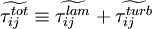
| (33) |
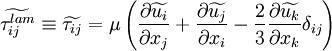
| (34) |
| (35) |
| (36) |
![\widetilde{q_j^{lam}} \equiv
\widetilde{q_j} \approx
- C_p \frac{\mu}{Pr} \frac{\partial \widetilde{T}}{\partial x_j} =
- \frac{\gamma}{\gamma-1} \frac{\mu}{Pr} \frac{\partial}{\partial x_j}
\left[ \frac{\overline{p}}{\overline{\rho}} \right]](/W/images/math/c/1/8/c186ac9836f5861e9f44e8e110b3ee53.png)
| (37) |
![\widetilde{q_j^{turb}} \equiv
C_p \overline{\rho u''_j T} \approx
- C_p \frac{\mu_t}{Pr_t} \frac{\partial \widetilde{T}}{\partial x_j} =
- \frac{\gamma}{\gamma-1} \frac{\mu_t}{Pr_t} \frac{\partial}{\partial x_j}
\left[ \frac{\overline{p}}{\overline{\rho}} \right]](/W/images/math/f/4/6/f46efa91ac350b21bd7d263841ed39f0.png)
| (38) |
| (39) |
If a separate turbulence model is used to calculate , and , and gas data is given for , and these equations form a closed set of partial differential equations, which can be solved numerically.
![\frac{\partial \rho}{\partial t} +
\frac{\partial}{\partial x_j}\left[ \rho u_j \right] = 0](/W/images/math/0/7/1/071e4f5508fd336ddad848551ce3188e.png)
![\frac{\partial}{\partial t}\left( \rho u_i \right) +
\frac{\partial}{\partial x_j}
\left[ \rho u_i u_j + p \delta_{ij} - \tau_{ji} \right] = 0](/W/images/math/6/f/c/6fc8041faa4be98ee72ec1e670fb22c7.png)
![\frac{\partial}{\partial t}\left( \rho e_0 \right) +
\frac{\partial}{\partial x_j}
\left[ \rho u_j e_0 + u_j p + q_j - u_i \tau_{ij} \right] = 0](/W/images/math/8/1/7/8176cdf87a72617542883cbbeafc50cc.png)