Two equation turbulence models
From CFD-Wiki
 model
model
 model
model
Two equation turbulence models are one of the most common types of turbulence models. Models like the k-epsilon model and the k-omega model have become industry standard models and are commonly used for most types of engineering problems. Two equation turbulence models are also very much still an active area of research and new refined two-equation models are still being developed.
By definition, two equation models include two extra transport equations to represent the turbulent properties of the flow. This allows a two equation model to account for history effects like convection and diffusion of turbulent energy.
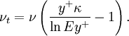
Most often one of the transported variables is the turbulent kinetic energy,  . The second transported variable varies depending on what type of two-equation model it is. Common choices are the turbulent dissipation,
  , or the Specific turbulence dissipation rate,
  . The second variable can be thought of as the variable that determines the scale of the turbulence (length-scale or time-scale), whereas the first variable, , determines the energy in the turbulence.
Contents |
Boussinesq eddy viscosity assumption
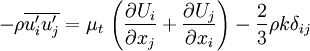
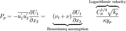
The basis for all two equation models is the Boussinesq eddy viscosity assumption, which postulates that the Reynolds stress tensor,  , is proportional to the mean strain rate tensor,
  , and can be written in the following way:
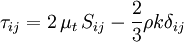
Where  is a scalar property called the eddy viscosity which is normally computed from the two transported variables. The last term is included for modelling incompressible flow to ensure that the definition of turbulence kinetic energy is obeyed:

The same equation can be written more explicitly as:
The Boussinesq assumption is both the strength and the weakness of two equation models. This assumption is a huge simplification which allows one to think of the effect of turbulence on the mean flow in the same way as molecular viscosity affects a laminar flow. The assumption also makes it possible to introduce intuitive scalar turbulence variables like the turbulent energy and dissipation and to relate these variables to even more intuitive variables like turbulence intensity and turbulence length scale.
The weakness of the Boussinesq assumption is that it is not in general valid. There is nothing which says that the Reynolds stress tensor must be proportional to the strain rate tensor. It is true in simple flows like straight boundary layers and wakes, but in complex flows, like flows with strong curvature, or strongly accelerated or decelerated flows the Boussinesq assumption is simply not valid. This gives two equation models inherent problems to predict strongly rotating flows and other flows where curvature effects are significant. Two equation models also often have problems to predict strongly decelerated flows like stagnation flows.
Near-wall treatments

The structure of turbulent boundary layer exhibits large, compared with the flow in the core region, gradients of velocity and quantities characterising turbulence. See introduction to wall bounded turbulent flows for more detail. In a collocated grid these gradients will be approximated using discretisation procedures which are not suitable for such high variation since they usually assume linear interpolation of values between cell centres.
Moreover, the additional quantities appearing in two-equation models require specification of their own boundary conditions that on purely physical grounds cannot be specified a priori.
This situation gave rise to a plethora of near-wall treatments. Generally speaking, two approaches can be distinguished:
- Low Reynolds number treatment (LRN)
- High Reynolds number treatment (HRN)
LRN integrates every equation up to the viscous sublayer and therefore the first computational cell must have its centroid in  . This results in very fine meshes close to the wall. Additionally, for some models additional treatment (damping functions) of equations is required to guarantee asymptotic consistency with the turbulent boundary layer behaviour. This often makes the equations stiff and further increases computation time.
HRN also known as wall functions approach relies on log-law velocity profile and therefore the first computational cell must have its centroid in the log-layer. Use of HRN enhances convergence rate and often numerical stability.
Interestingly, none of the current approaches can deal with buffer layer i.e. the layer in which both viscous and Reynolds stresses are significant. The first computational cell should be either in viscous sublayer or in log-layer -- not in-between. Automatic wall treatments, available in some codes, are an ad hoc solution but the blending techniques employed there are usually arbitrary and though they can achieve the switching between HRN and LRN treatments they cannot be regarded as the correct representation of the buffer layer.
There are two[1] possible ways of implementing wall functions in a finite volume code:
- Additional source term in the momentum equations.
- Modification of turbulent viscosity in cells adjacent to solid walls.
The source term in the first approach is simply the difference between logarithmic and linear interpolation of velocity gradient multiplied by viscosity (the difference between shear stresses). The second approach does not attempt to reproduce the correct velocity gradient. Instead, turbulent viscosity is modified in such a way as to guarantee the correct shear stress.
Standard wall functions
Using the compact version of log-law
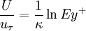 | (1) |
where  is equivalent to additive constants in the logarithmic law of the wall. Now using
  we obtain:
On the other hand, the linear interpolation for shear stress, rembembering that  , is:
, is:
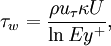
Comparing the above equations we obtain an expression for turbulent viscosity can be obtained:
 | (2) |
Note that  has been been incorporated in
  . The latter remains the only unknown in the equation and has to be estimated for the current velocity field. In the standard approach this cannot be done explicitly and instead an implicit way of obtaining
  has to be employed.
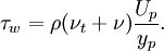
After multiplying log law (1) by  and after reorganising some terms we get:
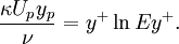 | (3) |
This equation can be solved numerically with respect to for example via root searching algorithms e.g. Newton method for specified  ,
,  and
and  . One iteration in a Newton method for (3) is
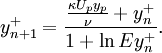
Thus obtained is then substituted to (2) Eventually the estimated serves also to define the values of turbulent quantities in the cell adjacent to the wall:

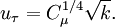
and for e.g. - model:
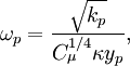
which are the values for and resulting from asymptotic analysis[2] of log layer. These wall functions for and are the results of the solution of model equation for the logarithmic layer.
The above methodology is known to produce spurious results in separated flows, where, by definition,  at the separation and reattachment point. Many extension of this approach has been proposed.
Launder-Spalding wall functions
This approaches utilises the relation
|
| (4) |
A three step procedure[3] is adopted:
- Calculate wall viscosity.
- Modify the production term in equation in the wall adjacent cell.
- Specify the value of the second variable in the wall adjacent cell.
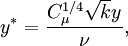
After substituing (4) to log law relation we obtain:
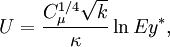
where
The production term (just in the first cell!) can be approximated as follows:
Lastly, we specify the remaining turbulence quantities in the same manner as in the previous approach.
See Also
References
- ↑ Bredberg, J. (2000), On the Wall Boundary Condition for Turbulence Models, Chalmers University of Technology Goteborg, Sweden
- ↑ Wilcox, D.C. (1993), Turbulence Modeling for CFD, DCW Industries, Inc.
- ↑ Launder, B.E. & D.B. Spalding (1974), "The numerical computation of turbulent flows", Computer Methods in Applied Mechanics and Engineering 3 (2): 269-289, ISSN 00457825