Calculation on non-orthogonal curvelinear structured grids, finite-volume method
From CFD-Wiki
(Difference between revisions)
(→2D case) |
(→2D case) |
||
| Line 37: | Line 37: | ||
</math> | </math> | ||
</td><td width="5%">(6)</td></tr></table> | </td><td width="5%">(6)</td></tr></table> | ||
| + | |||
| + | <table width="70%"><tr><td> | ||
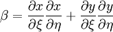
| + | :<math> | ||
| + | \beta = \frac{\partial x}{ \partial \xi} \frac{\partial x}{ \partial \eta} + \frac{\partial y}{ \partial \xi} \frac{\partial y}{ \partial \eta} | ||
| + | </math> | ||
| + | </td><td width="5%">(7)</td></tr></table> | ||
Revision as of 07:04, 18 August 2010
2D case
For calculations in complex geometries boundary-fitted non-orthogonal curvlinear grids is usually used.
General transport equation is transformed from the physical domain  into the computational domain
  as the following equation
|
| (2) |
![\frac{\partial}{\partial \xi} \left( \rho U \phi \right) + \frac{\partial }{ \partial \eta } \left( \rho V \phi \right) = \frac{\partial}{\partial \xi} \left[ \frac{\Gamma }{J} \left( \alpha \frac{\partial \phi}{\partial \xi} - \beta \frac{\partial \phi}{ \partial \eta} \right) \right] + \frac{\partial}{\partial \eta} \left[ \frac{\Gamma}{J} \left( \gamma \frac{\partial \phi}{\partial \eta} - \beta \frac{\partial \phi}{ \partial \xi} \right) \right] + J S^{\phi}](/W/images/math/3/8/2/382456ea15e881910f1b040f17a347bd.png)
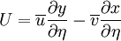
where
|
| (3) |
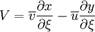
|
| (4) |
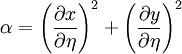
|
| (5) |
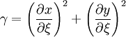
|
| (6) |
|
| (7) |