From CFD-Wiki
Introduction
The Cebeci-Smith [Cebeci and Smith (1967)] is a two-layer algebraic 0-equation model which gives the eddy viscosity,  , as a function of the local boundary layer velocity profile. The model is suitable for high-speed flows with thin attached boundary-layers, typically present in aerospace applications. Like the Baldwin-Lomax model, this model is not suitable for cases with large separated regions and significant curvature/rotation effects (see below). Unlike the Baldwin-Lomax model, this model requires the determination of of a boundary layer edge.
Equations
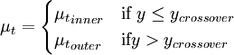
| (1) |
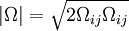
where  is the smallest distance from the surface where
  is equal to
  :
:

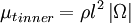
| (2) |
The inner region is given by the Prandtl - Van Driest formula:
| (3) |
where
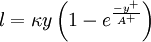
| (4) |
![\kappa = 0.4, A^+ = 26\left[1+y\frac{dP/dx}{\rho u_\tau^2}\right]^{-1/2}](/W/images/math/d/c/1/dc17c22b20b697ea91c81fe2827b5ef7.png)
| (5) |
| (5) |
| (6) |
The outer region is given by:

| (7) |
where  ,
,  is the velocity thickness given by
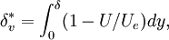
| (8) |
and  is the Klebanoff intermittency function given by
![F_{KLEB}(y;\delta) = \left[1 + 5.5 \left( \frac{y}{\delta} \right)^6
\right]^{-1}](/W/images/math/4/3/3/4331b74159c7e4947a91a3c15e2c8282.png)
| (10) |
Model variants
Performance, applicability and limitations
Implementation issues
References
- Smith, A.M.O. and Cebeci, T. Numerical solution of the turbulent boundary layer equations, Douglas aircraft division report DAC 33735.
- Wilcox, D.C. (1998), Turbulence Modeling for CFD, ISBN 1-928729-10-X, 2nd Ed., DCW Industries, Inc..