Baldwin-Lomax model
From CFD-Wiki
 model
model
 model
model
The Baldwin-Lomax model [Baldwin and Lomax (1978)] is a two-layer algebraic 0-equation model which gives the eddy viscosity,  , as a function of the local boundary layer velocity profile. The model is suitable for high-speed flows with thin attached boundary-layers, typically present in aerospace and turbomachinery applications. It is commonly used in quick design iterations where robustness is more important than capturing all details of the flow physics. The Baldwin-Lomax model is not suitable for cases with large separated regions and significant curvature/rotation effects (see below).
Contents |
Equations
|
| (1) |
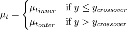
Where  is the smallest distance from the surface where
  is equal to
  :
:
|
| (2) |

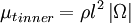
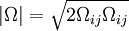
The inner region is given by the Prandtl - Van Driest formula:
|
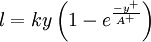
| (3) |
Where
|
| (4) |
|
| (5) |
|
| (6) |
The outer region is given by:
|
| (7) |

Where
|
| (8) |
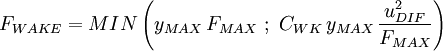
 and
and  are determined from the maximum of the function:
|
| (9) |
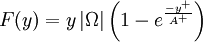
 is the intermittency factor given by:
|
| (10) |
![F_{KLEB}(y) = \left[1 + 5.5 \left( \frac{y \, C_{KLEB}}{y_{MAX}} \right)^6
\right]^{-1}](/W/images/math/9/b/d/9bde77641b7e232fa3e083d3e59795c4.png)
 is the difference between maximum and minimum speed in the profile. For boundary layers the minimum is always set to zero.
|
| (11) |

Model constants
The table below gives the model constants present in the formulas above. Note that  is a constant, and not the turbulence energy, as in other sections. It should also be pointed out that when using the Baldwin-Lomax model the turbulence energy, , present in the governing equations, is set to zero.
 |
 |
 |
 |
|
 |
| 26 | 1.6 | 0.3 | 0.25 | 0.4 | 0.0168 |
Model variants
In order to improve the Baldwin-Lomax model modifications of the model-constants can be made in order to account for the effect of adverse pressure gradients. This has been done by Granville and Turner and Jennions. For further information see the references below.
Performance, applicability and limitations
The Baldwin-Lomax model is suitable for high-speed flows with thin attached boundary layers. Typical applications are aerospace and turbomachinery applications. It is a low-Re model and as such it requires a fairly well-resolved grid near the walls, with the first cell located at  .
.
The model is popular in quick design-iterations due to its robustness and reliability. It seldom leads to any convergence problems and it seldom gives completely unphysical results.
The Baldwin-Lomax model should be used with great care in cases with large separations. It has been shown by several researchers that the Baldwin-Lomax model tends to overpredict separated regions (see for example the comments made by David Wilcox [Wilcox (1998)]). However, there are ad-hoc modifications which reduce this problem. For instance, prediction of separation is sensitive to the value of the coefficient and higher values than the original value tend to reduce the problems with too early separation. Also note that the Granville correction mentioned above, which attempts to account for adverse pressure gradient effects, increases the problem with too large separations.
The Baldwin-Lomax model does not account for the effect of a high free-stream turbulence level. Hence, it can not be used reliably when the free-stream turbulence has a signigicant effect on the boundary layer development.
Implementation issues
The computation of most of the model looks to relatively straightforward, but upon further examination, a few issues crop up. First, the model is nonlocal in nature due to the presence of the damping function. This means that for any location in the flow interior, we need a wall (or other suitable location) to compute a  from. Further, the calculation of and is best suited to a structured grid in which grid lines emanate outward from a wall (or wakeline, etc.). The model is thus best used in a structured grid setting, but has been used with unstructured grids via background grids [Mavriplis (1991)]. Second, the determination of and is sensitive to gridpoint location, as the vorticity magnitude is typically only available pointwise. One solution (perhaps with limited justification) is to do a fit of
  to reduce any problems. Finally, it is tempting to use the minimum of the two (inner and outer) eddy viscosity results instead of the correct crossover formula. This simplifies the programming, but is not justifiable on any other grounds (and can lead to the use of the wrong eddy viscosity). The (minimal) additional programming is required for correct model implementation.
We need some further information here about what to think about when implementing this model in a CFD code. For example, there are some issues when computing the max and min values in the formulas - in complex 3D cases you can sometimes find several local mins/maxs. Can anyone add something about this?
References
- Baldwin, B. S. and Lomax, H. (1978), "Thin Layer Approximation and Algebraic Model for Separated Turbulent Flows", AIAA Paper 78-257.
- Granville, P. S. (1987), "Baldwin-Lomax Factors for Turbulent Boundary Layers in Pressure Gradients", AIAA Journal, Vol. 25, No. 12, pp. 1624-1627.
- Mavriplis, D. J. (1991), "Algebraic turbulence modeling for unstructured and adaptive meshes", AIAA Journal, Vol. 29, pp. 2086-2093.
- Turner, M. G. and Jennions, I. K. (1993), "An Investigation of Turbulence Modeling in Transonic Fans Including a Novel Implementation of an Implicit
 Turbulence Model", Journal of Turbomachinery, Vol. 115, April, pp. 249-260.
- Wilcox, D.C. (1998), Turbulence Modeling for CFD, ISBN 1-928729-10-X, 2nd Ed., DCW Industries, Inc..
Return to Turbulence modeling