Discrete Poisson equation
From CFD-Wiki
In mathematics, the discrete Poisson equation is the finite difference analog of the Poisson equation. In it, the discrete Laplace operator takes the place of the Laplace operator. The discrete Poisson equation is frequently used in numerical analysis as a stand-in for the continuous Poisson equation, although it is also studied in its own right as a topic in discrete mathematics.
Contents |
On a two-dimensional rectangular grid
Using the finite difference numerical method to discretize the 2 dimensional Poisson equation (assuming a uniform spatial discretization) on an m x n grid gives the following formula:

where  and
and  . The preferred arrangement of the
solution vector is to use natural ordering which, prior to removing boundary elements, would look like:
. The preferred arrangement of the
solution vector is to use natural ordering which, prior to removing boundary elements, would look like:

This will result in an mn x mn linear system:
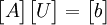
where
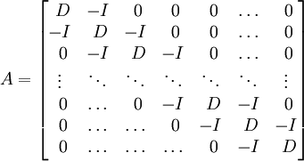
 is the m x m identity matrix, and
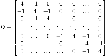
  , also m x m , is given by:
[1]
For each  equation, the columns of correspond to the
  components:

while the columns of to the left and right of correspond to the components:

and

respectively.
From the above, it can be inferred that there are  block columns of
  in
in  . It is important to note that prescribed values of (usually lying on the boundary) would have their corresponding elements removed from and . For the common case that all the nodes on the boundary are set, we have and , and the system would have the dimensions (m - 2) (n - 2) x (m - 2) (n - 2) , where and
would have dimensions (m-2) x (m-2) .
. It is important to note that prescribed values of (usually lying on the boundary) would have their corresponding elements removed from and . For the common case that all the nodes on the boundary are set, we have and , and the system would have the dimensions (m - 2) (n - 2) x (m - 2) (n - 2) , where and
would have dimensions (m-2) x (m-2) .
Example
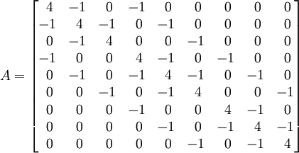
For a 5 x 5 (  and
and  ) grid with all the boundary nodes prescribed,
the system would look like:
) grid with all the boundary nodes prescribed,
the system would look like:

with
and
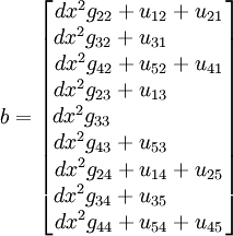
As can be seen, the boundary 's are brought to the right-hand-side
of the equation. [2] The entire system is 9 x 9
while and are 3 x 3 and given by:

and

Methods of Solution
Because  is block tridiagonal and sparse, many methods of solution
have been developed to optimally solve this linear system for
is block tridiagonal and sparse, many methods of solution
have been developed to optimally solve this linear system for  .
Among the methods are a generalized Thomas algorithm,
cyclic reduction, successive overrelaxation, and Fourier transforms. A theoretically optimal
.
Among the methods are a generalized Thomas algorithm,
cyclic reduction, successive overrelaxation, and Fourier transforms. A theoretically optimal  solution can be computed using multigrid methods.
Applications
In Computational fluid dynamics, for the solution of an incompressible flow problem, the incompressiblity condition acts as a constraint for the pressure. There is no explicit form available for pressure in this case due to a strong coupling of the velocity and pressure fields. In this condition, by taking the divergence of all terms in the momentum equation, one obtains the pressure poisson equation. For an incompressible "Flow" this constraint is given by:
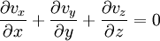
where  is the velocity in the
  direction,
  is
velocity in
is
velocity in  and
and  is the velocity in the
  direction. Taking divergence of the momentum equation and using the incompressibility constraint, the pressure poisson equation is formed given by:
where  is the kinematic viscosity of the fluid and
  is the velocity vector.
[3].
is the velocity vector.
[3].
Footnotes
- ↑ Golub, Gene H. and C.F. Van Loan, Matrix Computations, 3rd Ed., The Johns Hopkins University Press, Baltimore, 1996, pages 177-180.
- ↑ Cheny, Ward and David Kincaid, Numerical Mathematics and Computing 2nd Ed., Brooks/Cole Publishing Company, Pacific Grove, 1985, pages 443-448
- ↑ Fletcher, Clive A. J., Computational Techniques for Fluid Dynamics: Vol I, 2nd Ed., Springer-Verlag, Berlin, 1991, page 334-339.
References
- Cheny, Ward and David Kincaid, Numerical Mathematics and Computing 2nd Ed., Brooks/Cole Publishing Company, Pacific Grove, 1985.
- Golub, Gene H. and C.F. Van Loan, Matrix Computations, 3rd Ed., The Johns Hopkins University Press, Baltimore, 1996.
- Hoffman, Joe D., Numerical Methods for Engineers and Scientists, 4th Ed., McGraw-Hill Inc., New York, 1992.
- Sweet, Roland A., SIAM Journal on Numerical Analysis, Vol. 11, No. 3 , June 1974, 506-520.