Finite difference
From CFD-Wiki
In mathematics, a finite difference is like a differential quotient, except that it uses finite quantities instead of infinitesimal ones.
The derivative of a function f at a point x is defined by the limit
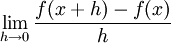 .
.
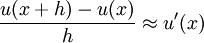
If h has a fixed (non-zero) value, instead of approaching zero, this quotient is called a finite difference.
Contents |
Calculus of finite differences
One important aspect of finite differences is that it is analogous to the derivative. This means that difference operators, mapping the function f to a finite difference, can be used to construct a calculus of finite differences, which is similar to the differential calculus constructed from differential operators.
Numerical analysis
Another important aspect is that finite differences approach differential quotients as h goes to zero. Thus, we can use finite differences to approximate derivatives. This is often used in numerical analysis, especially in numerical ordinary differential equations and numerical partial differential equations, which aim at the numerical solution of ordinary and partial differential equations respectively. The resulting methods are called finite-difference methods.
For example, consider the ordinary differential equation
The Euler method for solving this equation uses the finite difference
to approximate the differential equation by

The last equation is called a finite-difference equation. Solving this equation gives an approximate solution to the differential equation.
The error between the approximate solution and the true solution is determined by the error that is made by going from a differential operator to a difference operator. This error is called the discretization error or truncation error (the term truncation error reflects the fact that a difference operator can be viewed as a finite part of the infinite Taylor series of the differential operator).
Example: the heat equation
Consider the normalized heat equation in one dimension, with homogeneous Dirichlet boundary conditions:

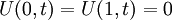 (boundary condition)
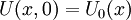 (initial condition)
One way to numerically solve this equation is to approximate all the derivatives by finite differences. We partition the domain in space using a mesh  and in time using a mesh
  . We assume a uniform partition both in space and in time, so the difference between two consecutive space points will be h and between two consecutive time points will be k. The points
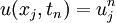
will represent the numerical approximation of 
Explicit method
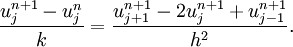
Using a forward difference at time  and a second-order central difference for the space derivative at position
  we get the recurrence equation:
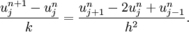
This is an explicit method for solving the one-dimensional heat equation.
We can obtain  from the other values this way:

where 
So, knowing the values at time n you can obtain the corresponding ones at time n+1 using this recurrence relation.  and
and  must be replaced by the border conditions, in this example they are both 0.
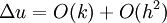
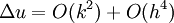
This explicit method is known to be numerically stable and convergent whenever  . The numerical errors are proportional to the time step and the square of the space step:
Implicit method
If we use the backward difference at time  and a second-order central difference for the space derivative at position we get the recurrence equation:
This is an implicit method for solving the one-dimensional heat equation.
We can obtain from solving a system of linear equations:

The scheme is always numerically stable and convergent but usually more numerically intensive than the explicit method as it requires solving a system of numerical equations on each time step. The errors are linear over the time step and quadratic over the space step.
Crank-Nicolson method
Finally if we use the central difference at time  and a second-order central difference for the space derivative at position we get the recurrence equation:

This formula is known as the Crank-Nicolson method.
We can obtain from solving a system of linear equations:

The scheme is always numerically stable and convergent but usually more numerically intensive as it requires solving a system of numerical equations on each time step. The errors are quadratic over the time step and formally are of the fourth degree regarding the space step:
(in reality, usually near the boundaries, the scheme failed to provide the fourth order accuracy over the space and degenerates to the quadratic errors).
Usually the Crank-Nicolson scheme is the most accurate scheme for small time steps. The explicit scheme is the least accurate and can be unstable, but is also the easiest to implement and the least numerically intensive. The implicit scheme works the best for large time steps.
References
- K.W. Morton and D.F. Mayers, Numerical Solution of Partial Differential Equations, An Introduction. Cambridge University Press, 2005.
- Oliver Rübenkönig, The Finite Difference Method (FDM) - An introduction, (2006) Albert Ludwigs University of Freiburg
- Finite Difference article on Wikipedia
- H. Lomax, T.H. Pulliam and D.W. Zingg, Fundamentals of Computational Fluid Dynamics, Series: Scientific Computation , Springer-Verlag, 2001, ISBN: 3-540-41607-2