Approximation Schemes for convective term - structured grids - Common
From CFD-Wiki
Discretisation Schemes for convective terms in General Transport Equation. Finite-Volume Formulation, structured grids
Introduction
This section describes the discretization schemes of convective terms in finite-volume equations. The accuracy, numerical stability, and boundedness of the solution depend on the numerical scheme used for these terms. The central issue is the specification of an appropriate relationship between the convected variable, stored at the cell center, and its value at each of the cell faces.
Basic Equations of CFD
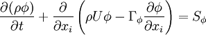
All the conservation equations can be written in the same generic differential form:
|
| (1) |

Equation (1) is integrated over a control volume and the following discretized equation for  is produced:
|
| (2) |
where  is the source term for the control volume
  , and
, and  and
and  represent, respectively, the convective and diffusive fluxes of across the control-volume face
 .
.
The convective fluxes through the cell faces are calculated as:
|
| (3) |
where  is the mass flow rate across the cell face . The convected variable
  associated with this mass flow rate is usually stored at the cell centers, and thus some form of interpolation assumption must be made in order to determine its value at each cell face. The interpolation procedure employed for this operation is the subject of the various schemes proposed in the literature, and the accuracy, stability, and boundedness of the solution depend on the procedure used.
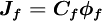
In general, the value of can be explicitly formulated in terms of its neighbouring nodal values by a functional relationship of the form:
|
| (4) |
where  denotes the neighbouring-node values.
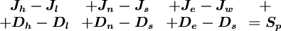
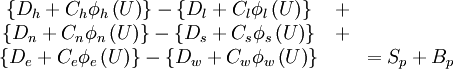
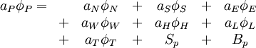
Combining equations (\ref{eq3}) through (\ref{eq4a}), the discretized equation becomes:
denotes the neighbouring-node values.
Combining equations (\ref{eq3}) through (\ref{eq4a}), the discretized equation becomes:
|
| (5) |
![\begin{matrix}
\left\{ D_{h} + C_{h} \left[ P \left( \phi_{nb} \right) \right]_{h} \right\} & - &
\left\{ D_{l} + C_{l} \left[ P \left( \phi_{nb} \right) \right]_{l} \right\} & + & \\
\left\{ D_{n} + C_{n} \left[ P \left( \phi_{nb} \right) \right]_{n} \right\} & - &
\left\{ D_{s} + C_{s} \left[ P \left( \phi_{nb} \right) \right]_{s} \right\} & + & \\
\left\{ D_{e} + C_{e} \left[ P \left( \phi_{nb} \right) \right]_{e} \right\} & - &
\left\{ D_{w} + C_{w} \left[ P \left( \phi_{nb} \right) \right]_{w} \right\} & = S_{p}
\end{matrix}](/W/images/math/3/a/0/3a0aa234abeb4cb4f2f309fac543a83c.png)
Convection Schemes
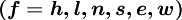
All of the convection schemes involve a stencil of cells in which the values of will be used to construct the face value

Where flow is from left to right, and is the face in question.
 - mean Upstream node
 - mean Central node
 - mean Downstream node
In the first plot, it is not so natural to think of the central node "C" not as the present node "P". It may be thought as the first node to the upstream direction of the surface in question .
Basic Discretisation schemes
Central Differencing Scheme (CDS)
It also can be considered as linear interpolation.
The most natural assumption for the cell-face value of the convected variable would appear to be the CDS, which calculates the cell-face value from:
|
| (6) |
or for more common case:
|
| (7) |

where the linear interpolation factor is definied as:
|
| (8) |
normalized variables - uniform grids
|
| (9) |
normalized variables - non-uniform grids
|
| (10) |
![\hat{\phi}_f = \left[ \left( 1-C_2 \right) \hat{\phi}_C + C_2 \right] U^{+}_{f} + \left[ C_2 \hat{\phi}_D + \left( 1 - C_2 \right) \right] U^{-}_{f}](/W/images/math/7/c/4/7c46e151a006e2627afa43891257664e.png)
This scheme is 2nd-order accurate, but is unbounded so that non-physical oscillations appear in regions of strong convection, and also in the presence of discontinuities such as shocks. The CDS may be used directly in very low Reynolds-number flows where diffusive effects dominate over convection.

Upwind Differencing Scheme (UDS) also (First-Order Upwind - FOU)
The UDS assumes that the convected variable at the cell face is the same as the upwind cell-centre value:
|
| (11) |

normalised variables
|
| (12) |

The UDS is unconditionally bounded and highly stable, but as noted earlier it is only 1st-order accurate in terms of truncation error and may produce severe numerical diffusion. The scheme is therefore highly diffusive when the flow direction is skewed relative to the grid lines.
|
| (13) |

|
| (14) |
UDS may be written as
|
| (15) |
or in more general form
|
| (16) |
where
|
| (17) |
|
| (18) |

Hybrid Differencing Scheme (HDS also HYBRID)
The HDS of Spalding [1972] switches the discretization of the convection terms between CDS and UDS according to the local cell Peclet number as follows:
|
| (19) |

|
| (20) |
The cell Peclet number is defined as:
|
| (21) |
in which  and are respectively, the cell-face area and physical diffusion coefficient. When
  ,CDS calculations tends to become unstable so that theHDS reverts to the UDS. Physical diffusion is ignored when .
The HDS scheme is marginally more accurate than the UDS, because the 2nd-order CDS will be used in regions of low Peclet number.
D.B.Spalding (1972), "A novel finite-difference formulation for different expressions involving both first and second derivatives", Int. J. Numer. Meth. Engng., 4:551-559, 1972.
Power-Law Scheme (also Exponential scheme or PLDS )
- Patankar, S. V. (1980), Numerical Heat Transfer and Fluid Flow, ISBN 0070487405, McGraw-Hill, New York.
High Resolution Schemes (HRS)
Classification of High Resolution Schemes
HRS can be classified as linear or non-linear, where linear means their coefficients are not direct functions of the convected variable when applied to a linear convection equation. It is important to recognise that linear convection schemes of 2nd-order accuracy or higher may suffer from unboundedness, and are not unconditionally stable.
Non-linear schemes analyse the solution within the stencil and adapt the discretisation to avoid any unwanted behavior, such as unboundedness (see Waterson [1994]). These two types of schemes may be presented in a unified way by use of the Flux-Limiter formulation (Waterson and Deconinck [1995]), which calculates the cell-face value of the convected variable from:
|
| (22) |

where  is termed a limiter function and the gradient ratio
  is defined as:
|
| (23) |

The generalisation of this approach to handle non-uniform meshes has been given by Waterson [1994]
Please note that linear does not mean first order
Linear schemes
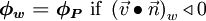
Linear schemes are those for which  is a linear function of
 is upwind differencing (first-order accurate)
 is central differencing (second-order accurate)
Kappa-formulation, Kappa-Schemes and Other schemes
kappa-formulation
B. van Leer (1985), "Upwind-difference methods for aerodynamics problems governed by the Euler equations", Lectures in Appl. Math., 22:327-336.
Higher order schemes are usually members of the  class, for which
|
| (24) |
![\varphi \left( r \right) = 0.5 \left[ \left( 1 + \kappa \right) r + \left( 1 - \kappa \right) \right]](/W/images/math/5/7/4/5740f8879092eb9cad6c0a6377905bd9.png)
Using this equation face variables can be expressed:
in usual variables
|
| (25) |
![\phi_{f}=\phi_{C}+ \frac{1}{4}\left[\left( 1+\kappa \right)\left(\phi_{D}-\phi_{C}\right)+\left(1-\kappa \right) \left( \phi_{D}-\phi_{U} \right)\right]](/W/images/math/0/0/c/00cce4f3c8f2da104ba303f077fb937f.png)
in normalised variables
|
| (26) |
![\hat{\phi_{f}}=\hat{\phi_{C}}+\frac{1}{4}
\left[\left( 1+\kappa \right)\left( 1-\hat{\phi_{C}}\right)+
\left( 1-\kappa \right)\hat{\phi_{C}}\right]](/W/images/math/c/3/a/c3a3cb90d7bfdc9f3b1041347cacde33.png)
The main schemes are

CDS (central differencing scheme) 
QUICK (quadratic upwind scheme) LUS (linear upwind scheme) Fromm CUS (cubic upwind scheme)


Non-Linear schemes
Non-linear schemes are those for which is not a linear function of . They fall into three categories, depending on the linear schemes on which they are based.
-
 QUICK based:
SMART (Sharp and Monotonic Algorithm for Realistic Transport, piecewise linear, bounded)
|
| (27) |

H-QUICK (Harmonic Quadratic Upwind Interpolation Convective Kinetics, smooth)
|
| (28) |

UMIST (Upstream Monotonic Interpolation Scalar Transport, piecewise linear , bounded)
|
| (29) |

CHARM (Cubic Parabolic High Accuracy Resolution Method,smooth, bounded)
|
| (30) |

|
| (31) |

-
 Fromm based:
MUSCL (Monotonic Upwind Scheme for Conservation Laws, piecewise linear)
|
| (32) |

van Leer (smooth)
|
| (33) |

OSPRE (smooth)
|
| (34) |
van Albada (smooth)
|
| (35) |
-
 other:
Superbee (piecewise linear)
|
| (36) |

MinMod (piecewise linear)
|
| (37) |

- Waterson, N. P and Deconinck, H (1995), "A unified approach to the design and application of bounded high-order covection schemes", 9th Int. Conf. on Numerical Methods in Laminar and Turbulent Flow, Atlanta, USA, July 1995, Taylor and Durbetaki eds., Pineridge Press.
- Waterson, N. P. (1994), "Development of bounded high-order convection scheme for general industrial applications", Project Report 1994-33, von Karman Institute for Fluid Dynamics, Sint-Genesius-Rode, Belgium.
Numerical Implementation of HRS (Deffered correction procedure)
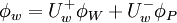
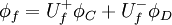
The HRS schemes can be introduced into equation (\ref{eq4b}) by using the deferred correction procedure of Rubin and Khosla [1982]. This procedure expresses the cell-face value by:
|
| (1) |
where  is a higher-order correction which represents the difference between the UDS face value
  and the higher-order scheme value
  , i.e.
|
| (1) |
If equation (\ref{eq10a}) is substituted into equation (\ref{eq4b}), the resulting discretised equation is:
|
| (1) |
where  contains the the deferred-correction source terms, given by:
|
| (1) |

This treatment leads to a diagonally dominant coefficient matrix since it is formed using the UDS.
The final form of the discretized equation:
|
| (1) |
Subscript represents the current computational cell;  represent the six neighbouring cells, and
  represents the previous timestep (transisent cases only).
The coefficients contain the appropriate contributions from the transient, convective and diffusive terms in (\ref{eq1}).
P.K. Khosla and S.G. Rubin (1974), "A diagonally dominant second order accurate implicit scheme", Comput. Fluids, 2 207-209.
S.G.Rubin and P.K.Khoshla (1982), "Polynomial interpolation method for viscous flow calculations", J. Comp. Phys., Vol. 27, pp. 153.
Diagonal dominance criterion
Normalised Variables Formulation (NVF)
B.P.Leonard (1988), "Simple high-accuracy resolution program for convective modelling of discontinuities", International J. Numerical Methods Fluids, 8:1291-1318.


Normalised Variables Diagram (NVD)
According to Leonard [1988], for any (in general nonlinear) characteristics in the normalized variable diagram (see figure below):
- Passing through
 is necessary and sufficient for second-order accuracy
- Passing through with a slope of 0.75 (for a uniform grid) is necessary and sufficient for third-order accuracy
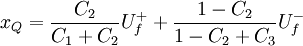
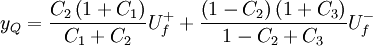
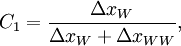
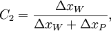
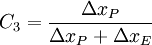
The horizontal and vertical coordinates of point in the normalized variable diagram, and the slope of the characteristics at the point for preserving the third-order accuracy for a nonuniform grid, can be obtained by simple algebra using eqs. [.....]
|
| (1) |
|
| (1) |
|
| (1) |

where
|
| (1) |
|
| (1) |
|
| (1) |
For a uniform qrid, 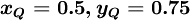 and
and 
Normalised variable diagram for various well-known schemes

Normalised Variable and Space Formulation (NVSF)
Darwish M.S. and Moukalled F. (1994), "Normalized Variable and Space Formulation Methodology for High-Resolution Schemes", Num. Heat Trans., part B, vol. 26, pp. 79-96.
Alves M.A., Cruz P. Mendes A. Magahaes F.D. Pinho F.T., Oliveira P.J. (2002), "Adaptive multiresolution approach for solution of hyperbolic PDEs", Computational Methods in Applied Mechanics and Engineering, 191, 3909-3928.

Convection Boundedness Criterion (CBC)
Choi S.K., Nam H.Y. and Cho M. (1995), "A comparison of high-order bounded convection schemes", Computational Methods in Applied Mechanics and engineering, Vol. 121, pp. 281-301.
Gaskell P.H. and Lau A.K.C. (1988), "Curvative-compensated convective transport: SMART, a new boundedness-preserving trasport algorithm", International Journal for Numerical Methods in Fluids, Vol. 8, No. 6, pp. 617-641.
Gaskel and Lau have formulated the CBC as follows. A numerical approximation to  is bounded if:
- for
 ,
,  is bounded below by the function
  and above by unity and passes through the points (0,0) and (1,1)
- for
 or
or  , is equal to
The CBC is clearly illustrated in figure below, where the line and the shaded area are the region over which the CBC is valid. The importance of the CBC is to provide a sufficient and necessary condition for guaranteeing the bounded solution if at most three neighbouring nodal values are used to approximate face values. It is well known that the positivity of finite-difference coefficients is also a sufficient condition for boundedness, but this is overly stringent, for the existense of negative coefficients does not neccesarily lead to over- or undershoots.

S.K. Godunov theorem
Monotonicity Criterion
Total Variation Diminishing (TVD)- Simplified Description
General issues
- A. Harten (1984), "On a class of high resolution total-variation stable finite difference schemes", SIAM J. Num. Analysis, 21, p1.
- A. Harten (1983), "High resolution schemes for hyperbolic conservation laws", J. Comput. Phys., 49:357-393, 1983.
- P. K. Sweby (1984), "High resolution schemes using flux-limiters for hyperbolic conservation laws", SIAM J. Num. Analysis, 21, p995.
TVD criterion
- no new local extrema must be created
- the value of an existing local minimum must be non-decreasing and that of the local maximum must be non-increasing
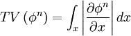
Total Variation (TV) of a function is defined by
|
| (1) |
Total Variation (TV) of a numerical solution is defined by
|
| (1) |
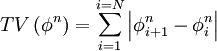
where  - grid point index
for a set of discrete data 

the TV is defined by
|
| (1) |

|
| (1) |

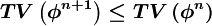
For monotonicity to be satisfied, this TV must not be increased!
Finally a numerical scheme is said to be TVD if:
|
| (1) |
where  - time step or iteration index
Using normalised varibles, TVD condition cab be written:
|
| (1) |
![\hat{\phi_{C}} \leq \hat{\phi_{f}} \leq 2\hat{\phi_{C}} , \hat{\phi_{f}} \leq 1 \ \ \mbox{for} \ \ \hat{\phi_{C}} \in \left[ 0,1 \right]](/W/images/math/f/0/c/f0cc57ee11e3aea517991dfd18efb072.png)
|
| (1) |
![\hat{\phi_{f}} = \hat{\phi_{C}} \ \ \mbox{for} \ \ \hat{\phi_{C}} \notin \left[ 0,1 \right]](/W/images/math/a/d/0/ad0497ee9b995907f239868f7bc30bf3.png)
To obtain differencing scheme, satisfying TVD condition, flux limiter is included, which depends upon function's gradients.
In order to provide monotonicity of the solution, it is necessary to implement condition [K. Fletcher]
|
| (1) |

where
|
| (1) |
![\mbox{minmod} \left( x , y \right) = \frac{1}{2} \left[ \mbox{sign} \left(x \right) + \mbox{sign} \left(y \right) \right] \min \left( \left| x \right|, \left| y \right| \right)](/W/images/math/e/b/9/eb95322717eae7e5fd821acad355e120.png)
Total Variation Diminishing Diagram (Sweby diagram)
Flux-limiting formulation

Discretization schemes Quality Criterions
Return to Numerical Methods
Return to Approximation Schemes for convective term - structured grids