Code: Thermal cavity using pressure-free velocity form
From CFD-Wiki
Thermal cavity using pressure-free velocity formulation
This sample code uses four-node quartic Hermite finite elements for velocity and simple-cubic Hermite elements for the temperature and pressure, and uses simple and iteration.
Theory
The incompressible Navier-Stokes equation is a differential algebraic equation, having the inconvenient feature that there is no explicit mechanism for advancing the pressure in time. Consequently, much effort has been expended to eliminate the pressure from all or part of the computational process. We show a simple, natural way of doing this.
The incompressible Navier-Stokes equation is composite, the sum of two orthogonal equations,
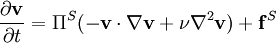 ,
,
 ,
,
where  and
and  are solenoidal and irrotational projection operators satisfying
  and
and
 and
and  are the nonconservative and conservative parts of the body force. This result follows from the Helmholtz Theorem . The first equation is a pressureless governing equation for the velocity, while the second equation for the pressure is a functional of the velocity and is related to the pressure Poisson equation. The explicit functional forms of the projection operator in 2D and 3D are found from the Helmholtz Theorem, showing that these are integro-differential equations, and not particularly convenient for numerical computation.
Equivalent weak or variational forms of the equations, proved to produce the same velocity solution as the Navier-Stokes equation are
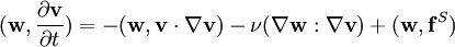 ,
,
 ,
,
for divergence-free test functions  and irrotational test functions
  satisfying appropriate boundary conditions. Here, the projections are accomplished by the orthogonality of the solenoidal and irrotational function spaces. The discrete form of this is emminently suited to finite element computation of divergence-free flow.
In the discrete case, it is desirable to choose basis functions for the velocity which reflect the essential feature of incompressible flow — the velocity elements must be divergence-free. While the velocity is the variable of interest, the existence of the stream function or vector potential is necessary by the Helmholtz Theorem. Further, to determine fluid flow in the absence of a pressure gradient, one can specify the difference of stream function values across a 2D channel, or the line integral of the tangential component of the vector potential around the channel in 3D, the flow being given by Stokes' Theorem. This leads naturally to the use of Hermite stream function (in 2D) or velocity potential elements (in 3D).
Involving, as it does, both stream function and velocity degrees-of-freedom, the method might be called a velocity-stream function or stream function-velocity method.
We now restrict discussion to 2D continuous Hermite finite elements which have at least first-derivative degrees-of-freedom. With this, one can draw a large number of candidate triangular and rectangular elements from the plate-bending literature. These elements have derivatives as components of the gradient. In 2D, the gradient and curl of a scalar are clearly orthogonal, given by the expressions,
![\nabla\phi = \left[\frac{\partial \phi}{\partial x},\,\frac{\partial \phi}{\partial y}\right]^T, \quad
\nabla\times\phi = \left[\frac{\partial \phi}{\partial y},\,-\frac{\partial \phi}{\partial x}\right]^T.](/W/images/math/8/a/5/8a58150cd07872905de0f26ea5212055.png)
Adopting continuous plate-bending elements, interchanging the derivative degrees-of-freedom and changing the sign of the appropriate one gives many families of stream function elements.
Taking the curl of the scalar stream function elements gives divergence-free velocity elements [3][4][7]. The requirement that the stream function elements be continuous assures that the normal component of the velocity is continuous across element interfaces, all that is necessary for vanishing divergence on these interfaces.
Boundary conditions are simple to apply. The stream function is constant on no-flow surfaces, with no-slip velocity conditions on surfaces. Stream function differences across open channels determine the flow. No boundary conditions are necessary on open boundaries [3], though consistent values may be used with some problems. These are all Dirichlet conditions.
The algebraic equations to be solved are simple to set up, but of course are non-linear, requiring iteration of the linearized equations.
For the thermal cavity, an energy equation expressed in terms of the temperature is introduced, and when the temperature-dependent density changes are small, a temperature-dependent buoyancy force  is introduced into the velocity equation. One nondimensional form is,


where Ra is the Rayleigh number and Pr is the Prandtl number. The velocity and temperature equations are coupled through the buoyancy force. In the following code we choose to split the equations. Instead of solving the coupled equations, which involves a larger matrix, we sequentially solve the steady nonlinear algebraic equations,


This results in smaller sets to be solved, but precludes using Newton's method to speed convergence. The solution of this pair is iterated until convegence.
The finite elements we will use here are a modified form of one due to Gopapacharyulu [1][2] and Watkins [5][6]. These quartic-complete elements have 24 degrees-of-freedom, six degrees-of-freedom at each of the four nodes, and have continuous first derivatives. In the sample code the modified form of the Hermite element was obtained by interchanging first derivatives and the sign of one of them. The degrees-of-freedom of the modified element are the stream function, two components of the solenoidal velocity, and three second derivatives of the stream function. The components of the velocity element, obtained by taking the curl of the stream function element, are continuous at element interfaces. Simple-cubic Hermite elements with three degrees-of-freedom are used for the temperature and pressure, though a simple bilinear element could be used for pressure.
The code implementing the thermal cavity problem is written for Matlab. The script below is problem-specific, and calls problem-independent functions to evaluate the velocity and thermal element diffusion and convection matricies, the buoyancy matrix, and to evaluate the pressure from the resulting velocity field. These six functions accept general convex quadrilateral elements with straight sides, as well as the rectangular elements used here. Other functions are a GMRES iterative solver using ILU preconditioning and incorporating the essential boundary conditions, and a function to produce non-uniform nodal spacing for the problem mesh.
This "educational code" is a simplified version of code used in [4]. The user interface is the code itself. The user can experiment with changing the mesh, the Rayleigh number, and the number of nonlinear iterations performed, as well as the relaxation factor, and there is an option for the nondimensional form of the temperature. There are suggestions in the code regarding near-optimum choices for this factor as a function of Rayleigh number. For larger Rayleigh numbers, a smaller relaxation factor speeds up convergence by smoothing the velocity in the factor  of the convection term, but will impede convergence if made too small.
The output consists of graphic plots of contour levels of the stream function, temperature, velocity components, the pressure levels, and convergence rate.
The simplified version for this Wiki resulted from removal of computation of the vorticity field, a restart capability, comparison with published data, and production of publication-quality plots from the research code used with the paper. The vorticity at the nodes can be found, of course, from the second derivatives of the stream function. This code can be extended to fifth-order elements (and generalized bicubic elements), which use the same degrees-of-freedom, by simply replacing the velocity class evaluating the elements.
This modified version posted 3/15/2013 updates the code to MatLab version R2012b. The element properties are now defined in classes, and the code has been modified to accept class definitions for additional cubic and quintic divergence-free elements on quadrilaterals and quadratic and quartic divergence-free elements on triangles.
Thermal cavity Matlab script
TC44SW            THERMAL-DRIVEN CAVITY
%
% Finite element solution of the 2D Navier-Stokes equation for the
%  bouyancy-driven thermal cavity problem using quartic Hermite elements
%   and SEGMENTED SOLUTIONS (T-V split).
%
% This could be characterized as a VELOCITY-STREAM FUNCTION or
%   STREAM FUNCTION-VELOCITY method.
%
% Reference:  "Computation of incompressible thermal flows using Hermite finite
%    elements", Comput. Methods Appl. Mech. Engrg, 199, P3297-3304 (2010).
%
% Simplified Wiki version
%
% The rectangular problem domain is defined between Cartesian
%   coordinates Xmin & Xmax and Ymin & Ymax.
% The computational grid has NumNx nodes in the x-direction
%   and NumNy nodes in the y-direction.
% The nodes and elements are numbered column-wise from the
%   upper left corner to the lower right corner.
% Segregated version
%
%This script direcly calls the user-defined functions:
%  ELS4424r      - class with definitions of velocity shape functions
%  ELG3412r      - class with definitions of temperature & pressure fns
%  regrade       - to regrade the mesh (optional)
%  DMatW         - to evaluate element velocity diffusion matrix
%  CMatW         - to evaluate element velocity convection matrix
%  TDMatSW       - to evaluate element thermal diffusion matrix
%  TCMatSW       - to evaluate element thermal convection matrix
%  BMatSW        - to evaluate element bouyancy matrix
%  GetPres3W     - to evaluate the pressure
%
% Uses:
%   ilu          - incomplete LU preconditioner for solver
%   gmres        - sparse linear solver to solve the sparse system
% Indirectly uses:
%   Gquad2       - Gauss integraion rules
%   ELG3412r     - class of pressure basis functions
%
% Jonas Holdeman,   December 2008   revised March 2013
 ............
Program script for thermal cavity with pressure-free velocity method (TC44SW.m)
Modified-quartic velocity class for pressure-free velocity method (ELS4424r.m)
Simple-cubic pressure class for pressure-free velocity method (ELG3412r.m)
Velocity diffusion matrix for pressure-free velocity method (DMatW.m)
Velocity convection matrix for pressure-free velocity method (CMatW.m)
Thermal diffusion matrix for pressure-free velocity method (TDMatSW.m)
Thermal convection matrix for pressure-free velocity method (TCMatSW.m)
Buoyancy matrix for pressure-free velocity method (BMatSW.m)
Consistent pressure for pressure-free velocity method (GetPres3W.m)
Grade node spacing (regrade.m)
references
[1] Gopalacharyulu, S. (1973), "A higher order conforming rectangular plate element", Int. J. Numer. Meth. Fluids, 6: 305-308.
[2] Gopalacharyulu, S. (1976), "Author's reply to the discussion by Watkins", Int. J. Numer. Meth. Fluids, 10: 472-474.
[3] Holdeman, J. T. (2010), "A Hermite finite element method for incompressible fluid flow", Int. J. Numer. Meth. Fluids, 64: 376-408.
[4] Holdeman, J. T. and Kim, J.W. (2010), "Computation of incompressible thermal flows using Hermite finite elements", Comput. Methods Appl. Mech. Engr., 199: 3297-3304.
[5] Watkins, D. S. (1976), "A comment on Gopalacharyulu's 24 node element", Int. J. Numer. Meth. Fluids, 10: 471-472. }}
[6] Watkins, D. S. (1976), "On the construction of conforming rectangular plate elements", Int. J. Numer. Meth. Fluids, 10: 925-933. }}
[7] Holdeman, J. T. (2012), "A velocity-stream function method for three-dimensional incompressible fluid flow", Comput. Methods Appl. Mech. Engr., 209-212: 66-73.