Introduction to turbulence/Homogeneous turbulence
From CFD-Wiki
| Nature of turbulence |
| Statistical analysis |
| Reynolds averaged equation |
| Turbulence kinetic energy |
| Stationarity and homogeneity |
| Homogeneous turbulence |
| Free turbulent shear flows |
| Wall bounded turbulent flows |
| Study questions
... template not finished yet! |
A first look at decaying turbulence
Look, for example, at the decay of turbulence which has already been generated. If this turbulence is homogeneous and there is no mean velocity gradient to generate new turbulence, the kinetic energy equation reduces to simply:
|
| (1) |

This is often written (especially for isotropic turbulence) as:
|
| (2) |
![\frac{d}{dt} \left[ \frac{3}{2} u^{2} \right] = - \epsilon](/W/images/math/a/c/2/ac251958c2df0a8a260f8f83d2645da2.png)
where
|
| (3) |

Now you can't get any simpler than this. Yet unbelievably we still don't have enough information to solve it. Let's try. Suppose we use the extanded ideas of Kolmogorov we introduced in Chapter 3 to related the dissipation to the turbulence energy, say:
|
| (4) |
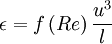
Already you can see we have two problems, what is  , and what is the time dependece of
  ? Now there is practically a different answer to these questions for every investigator in turbulence - most of whom will assure you their choice is only reasonable one.
Figure 6.1 shows an attempt to correlate some of the grid turbulence data using the longitudinal integral scale for , i.e.,  , or simply
  . The first thing you notice is the problem at low Reynolds number. The second is probably the possible asymptote at the higher Reynolds numbers. And the third is probably the scatter in the data, which is characteristic of most turbulence experiments, especially if you try to compare the results of one experiment to the other.
Let's try to use the apparent asymptote at high Reynolds number to our advantage by arguing that  , where
  is a constant. Note that this limit is consistent with the Kolmogorov argument we made back when we were talking about the dissipation earlier, so we might feel on pretty firm ground here, at least at high turbulent Reynolds numbers. But before we feel too comfortable about this, let's look at another curve shown in figure 6.2. This one is also due to Sreenivasan, but a compiled a decade later and based on large scale computer simulations of turbulence. There is less scatter, but it appears that the asymptote depends on the details of how the experiment was forced at the large scales of motion. This is not good, since it means that the answer depends on the particular flow - exactly what we wanted to avoid by modelling in the first place.
Nonetheless, let's proceed by assuming in spite of the evidence that  and is the integral scale. Now how does vary with time? Figure 6.3 shows the ration of the integral scale to the Taylor microscale from the famous Comte-Bellot/Corrsin (1971) experiment. One might assume, with some theoretical justification, that
 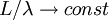 . This would be nice since you will be able to show that if the turbulence decays as a power law in time, say
  , then
  . But as shown in Figure 6.4 from Wang et all (2000), this is not very good assumption for the DNS data avialable at this time. Now I believe this is because of problems in the simulations, mostly having to do with the fact that turbulence in a box is not a very good approximation for truly homogeneous turbulence unless the size of the box is much larger than the energetic scales. Figure 6.5 shows what happens if you try to correct for the finite box size, and now the results look pretty good.
So the bottom line is that we don't really know yet for sure how behaves with time, or even whetherwe should have confidence in the expiremental and DNS attempts to determine it. Regardless, most assume that varies as a power of time, say  . There are various justifications for this and everyone has his own choice for
  , but the truth is that the main justification is that it allows us to solve the equation/ In fact it is easy to show by substitution that this implies directly that the energy decays as a power law in time; in fact:
|
| (5) |

You can see immediately that if I am right and 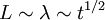 then
then  . Now any careful study of the data will convince you that the energy indeed decays as a power law in time, but there is no question that
  , but
, but  , at least for most of the experiments. Most people have tried to fix this problem changing . But I say the problem is in and the assumption that
  at finite Reynolds numbers. I would argue that
  only in the limit of infinite Reynolds number.
To see why I believe this, try doing the problem another way. We know for sure that if the turbulence decays as a power law, then the Taylor microscale,  , must be proportional exactly to
  . Thus we must have (assuming isotropy):
|
| (6) |
It is easy to show that  where
where  is gyven by:
|
| (7) |

and any value of  is acceptable. Obviosly the difference lies in the use of the relation
  at finite Reynolds numbers.
Believe it or not, this whole subject is one of the really hot debates of the last decade, and may well be for the next as well. Who knows, maybe some of you will be involved in resolving it, since it really is one of the most fundamental qustions in turbulence.
The dissipation equation and turbulence modelling
If you are really more inclined toward engineering than physics, you might be wondering whether the ambiguities above make any difference. They might. And in fact they might lie at the core of the reasons why we can't do things better with our existing single point turbulence models. To see this let's consider the dissipation equation.
The derivation of this equation begins by taking the gradient of the equation for the fluctuating velocity, then interchanging the order of the time and space derivatives to get it into an equation for the fluctuating strain-rate, then averaging and multiplying by twice the kinematic viscosity to obtain an equation for the dissipation of kinetic energy per unit mass due to the fluctuating velocity field. After some rearrangement the result is:
A second look at simple shear flow turbulence
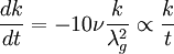
Let's consider another homogeneous flow that seems pretty simple at first sight, homogeneous shear flow turbulence with constant mean shear. We already considered this flow when we were talking about the role of the pressure-strain rate terms. Now we will only worry, for the moment, about the kinetic energy which reduces to:
|
| (8) |
![\frac{\partial }{\partial t} \left[ \frac{1}{2} k \right] = - \left\langle uv \right\rangle \frac{d U}{d y} - \epsilon](/W/images/math/3/d/1/3d167fcb8da6667620a699d420e11914.png)
Now turbulence modellers (and most experimentalists as well) would love for the left-hand side to be exactly zero so that the production and dissipation exactly balance. Unfortunately Mother Nature, to this point at least, has not allowed such flow to be generated. In every experiment to-date, the energy increases with time (or equivalently, down the tunnel).
Let's make a few simple assumptions and see if we can figure out what is going on. Suppose we assume that the correlation coefficient  is a constant. Now, we could again assume that
  , at least in the very high Reynolds number limit. But for reasons that will be obvious below, let's assume something else we know for sure about the dissipation; namely that:
|
| (9) |

where  is the Taylor microscale and
  (exact for isotropic turbulence). Finally let's assume that the mean shear is constant so
  is constant also. Then our problem simplifies to:
|
| (10) |
Even with all these simplifications and assumptions the problem still comes down to "What is  ?". Now the one thing that all the experiments agree on is that
  is approximately constant. (I actually have a theory about this, together with M.Gibson, and it even predicts this result.) Now you have all you need to finish the problem, and I will leave it for you. But when you do you will find that the turbulence grows (or decays) exponentialy. How fast it grows(or decays) depends on the ratio of the production to dissipation; i.e.,
|
| (11) |
My personal belief is that  depends on the upstream or initial conditions, the closer is to unity. If I am right, then you will only get
  as an infinite Reynolds number limit. Which in turn implies you can never really achieve the ideal flow many people would like where the productions and dissipation exactly balance.