Solution of Boltzmann Equation
From CFD-Wiki
Definition
Consider the classical Boltzmann equation for a simple, dilute gas of particles

which describes the time evolution of the particle density 
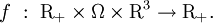
Here  denotes the set of non-negative real numbers and
  is a domain in physical space. The right-hand side of the Boltzmann equation, known as the collision integral or the collision term, is of the form
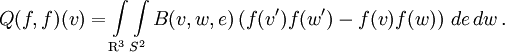
where
 are the pre-collision velocities,
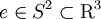 is a unit vector,
 are the post-collision velocities and
 is the collision kernel. The operator
  represents the change of the distribution function due to the binary collisions between particles. A single collision
results in a change of the velocities of the colliding partners
represents the change of the distribution function due to the binary collisions between particles. A single collision
results in a change of the velocities of the colliding partners 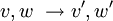 with
with
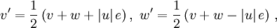
where  denotes the relative velocity. The Boltzmann equation is subjected to an initial condition

and to the boundary conditions on  .
.
The kernel can be written as

The function ![\sigma\,:\,{\rm R}_+\times [-1,1] \rightarrow {\rm R}_+](/W/images/math/c/6/b/c6bac89026f7bdaef4da6a891d43c0e7.png) is the differential cross-section and
is the differential cross-section and  is the scattering angle.
One of the first discrete versions of the Boltzmann equation was published by D. Goldstein, B. Sturtevant and J.E. Broadwell. Many authors then published different ideas to lead to a discrete version of the Boltzmann collision operator Rogier, Schneider in 1994; Ohwada in 1993, Wagner in 1995, Platkowski, Illner in 1988, Palczewski, Schneider in 1998, Panferov in 1997, Panferov, Heintz in 2002.
The main difficulty with the deterministic approximation of the Boltzmann collision integral besides its
high dimensionality is the fact that any grid for the integration over the whole space  will not fit for the integration over the unit sphere
  . Thus only
  irregularly distributed integration points belong to the unit sphere if
  regular points in one direction are used for the approximation of the integral.
A. Bobylev, A. Palczewski and J. Schneider in 1995 considered this direct approximation of the Boltzmann collision integral and showed that the corresponding numerical method is consistent. The arithmetical work is  per time step and the formal accuracy is
  .
.
L. Pareschi and B. Perthame in 1996 considered deterministic spectral methods for the Boltzmann equation and in 2000 L. Pareschi and G. Russo show that these method are consistent and are able to provide spectrally accurate solutions at  computational cost. Moreover the method are able to treat also the difficult case of non cut-off collision kernel as shown by L.Pareschi, G.Toscani and C.Villani in 2003.
Later, Ibragimov and Rjasanow in 2002, F.Filbet, L. Pareschi and G.Toscani in 2004 studied spectral methods for numerical solution of Boltzmann equations and Ibragimov, Rjasanow in 2002 proved an  numerical accuracy with arithmetic complexity.
Recent results that improve the numerical solution of Boltzmann equations are done in 2007 by Ibragimov and Ibragimova who suggests to use a multilinear approximation to approximate a velocity subspace. Hence, the function state  is approximated as one of the following methods:
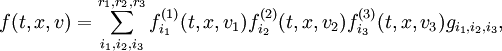
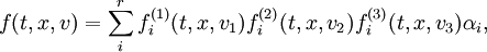
where  are almost constant.
Indeed, when are equal to 1, we can easily get Navies-Stocks equation, when ranks are equal to 2, we have very robust model for the boundary layer, with small enough rank (3-5) we can definitely explain a shock waves, etc.
Several real time industrial applications solved with the help of this method are mentioned on the web site of Elegant Mathematics who develops such solvers and provide test calculations for free.
Finally let us mention that an algorithm which strongly reduces the computational cost of spectral methods to  in the 3D case for hard spheres without loosing the spectral accuracy has been obtained recently by F.Filbet, C.Mouhot and L.Pareschi in 2006 and several applications of this method has been presented to show its potential in computing solution of CFD problems involving the Boltzmann equation.