V2-f models
From CFD-Wiki
Contents |
Introduction
The  model is similar to the Standard k-epsilon model. Additionally, it incorporates also some near-wall turbulence anisotropy as well as non-local pressure-strain effects. It is a general turbulence model for low Reynolds-numbers, that does not need to make use of wall functions because it is valid upto solid walls.
Instead of turbulent kinetic energy
model is similar to the Standard k-epsilon model. Additionally, it incorporates also some near-wall turbulence anisotropy as well as non-local pressure-strain effects. It is a general turbulence model for low Reynolds-numbers, that does not need to make use of wall functions because it is valid upto solid walls.
Instead of turbulent kinetic energy  , the model uses a velocity scale
  (hence the name or the v2-f model) for the evaluation of the eddy viscosity. can be thought of as the velocity fluctuation normal to the streamlines. It can provide the right scaling for the representation of the damping of turbulent transport close to the wall. The anisotropic wall effects are modelled through the elliptic relaxation function
  , by solving a separate elliptic equation of the Helmholtz type.
In order to improve the computational preformances of the  model, a variant of this eddy-viscosity model is derived when the change of variables is introduced.
Instead of using the wall-normal velocity fluctuation
model, a variant of this eddy-viscosity model is derived when the change of variables is introduced.
Instead of using the wall-normal velocity fluctuation  as the velocity scale, the normalised wall-normal velocity scale
  is used (hence the name
  or the zeta-f model).
This turbulence variable can be regarded as the ratio of the two time
scales: scalar
or the zeta-f model).
This turbulence variable can be regarded as the ratio of the two time
scales: scalar  (isotropic), and lateral
  (anisotropic).
Following the definition of
(anisotropic).
Following the definition of  , the new transport equation is derived from the equations for and , and solved instead of the transport equation for .
The equations
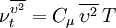
The turbulent viscosity is defined as
and the turbulent quantities, in addition to standard and  , are obtaned from two more equations: the transport equation for
![\frac{\partial \overline{\upsilon^2}}{\partial t} + U_j \frac{\partial \overline{\upsilon^2}}{\partial x_j} = k f - \frac{\overline{\upsilon^2}}{k} \varepsilon + \frac{\partial}{\partial x_j} \left[ \left( \nu + \frac{\nu_t}{\sigma_{\overline{\upsilon^2}}} \right) \frac{\partial \overline{\upsilon^2}}{\partial x_j} \right]](/W/images/math/4/d/f/4dfe2edd7e498f15491c4d78f266a9a3.png)
and the elliptic equation for the relaxation function
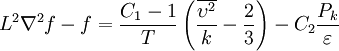
where the turbulence length scale 
![\displaystyle L = C_L \max \left[ \frac{\displaystyle k^{3/2}}{\displaystyle \varepsilon} , C_{\eta} \left( \frac{\displaystyle \nu^3}{\displaystyle \varepsilon} \right)^{1/4} \right]](/W/images/math/e/1/3/e1346b0f44e1e583315e145067993987.png)
and the turbulence time scale 
![\displaystyle T = \max \left[ \frac{\displaystyle k}{\displaystyle \varepsilon} , C_T \left( \frac{\displaystyle \nu}{\displaystyle \varepsilon} \right)^{1/2} \right]](/W/images/math/3/4/5/345e881f3c23753ab889f271376c958f.png)
are bounded with their respective the Kolmogorov definitions (realisability constraints can also be applied, as given below).
The coefficients used read:  ,
,  ,
,  ,
,  ,
,  ,
,  and
and  .
.
The equations
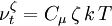
The turbulent viscosity is defined as
and the turbulent quantities are obtained from another set of equations. When the change of variables is done, the obtained transport equation for reads
![\frac{\partial \zeta}{\partial t} + U_j \frac{\partial \zeta}{\partial x_j} = f - \frac{\zeta}{k} P_k + \frac{\partial}{\partial x_j} \left[ \left( \nu + \frac{\nu_t}{\sigma_{\zeta}} \right) \frac{\partial \zeta}{\partial x_j} \right]](/W/images/math/1/4/3/143979f772a60676f05d24a868fa7f47.png)
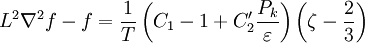
and, in conjunction with the quasi-linear SSG pressure-strain model, the elliptic equation for the relaxation function
where the turbulence time scale
![T = \max \left[ \min \left( \frac{k}{\varepsilon},\, \frac{0.6}{\sqrt{6} C_{\mu} |S|\zeta} \right), C_T \left( \frac{\nu}{\varepsilon} \right)^{1/2} \right]](/W/images/math/d/7/0/d706d5a17f5d2819e1861d7f20beed45.png)
and the turbulence length scale
![L = C_L \, \max \left[ \min \left( \frac{k^{3/2}}{\varepsilon}, \,
\frac{k^{1/2}}{\sqrt{6} C_{\mu} |S| \zeta} \right), C_{\eta}
\left( \frac{\nu^3}{\varepsilon} \right)^{1/4} \right]](/W/images/math/7/a/9/7a9caac33babd65efcae68be6079981a.png)
are limited with their Kolmogorov values as the lower bounds, and Durbin's realisability constraints.
The coefficients used read: ,  , ,
, ,  , ,
, ,  and .
and .
Notes
This model can not be used to solve Eulerian multiphase problems.
Mathematically and physically the and the model are the same, but due to better numerical properties (stability and near-wall mesh requirements) the model performs better in the complex flow calculations.
References
- Durbin, P. Separated flow computations with the
 model, AIAA Journal, 33, 659-664, 1995.
- Laurence, D.R., Uribe J.C., Utyuzhnikov, S.V. A Robust Formulation of the v2-f Model, Flow Turbulence and Combustion, 73, 169-185, 2004.
- Popovac, M., Hanjalic, K. Compound Wall Treatment for RANS Computation of Complex Turbulent Flows and Heat Transfer, Flow Turbulence and Combustion, 78, 177-202, 2007.