Spalart-Allmaras model
From CFD-Wiki
 model
model
 model
model
Spalart-Allmaras model is a one equation model which solves a transport equation for a viscosity-like variable  . This may be referred to as the Spalart-Allmaras variable.
Contents |
Original model
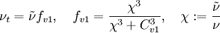
The turbulent eddy viscosity is given by
![\begin{matrix}
\frac{\partial \tilde{\nu}}{\partial t} + u_j \frac{\partial \tilde{\nu}}{\partial x_j} & = & C_{b1} [1 - f_{t2}] \tilde{S} \tilde{\nu} + \frac{1}{\sigma} \{ \nabla \cdot [(\nu + \tilde{\nu}) \nabla \tilde{\nu}] + C_{b2} | \nabla \tilde{\nu} |^2 \} - \\
\ & \ & \left[C_{w1} f_w - \frac{C_{b1}}{\kappa^2} f_{t2}\right] \left( \frac{\tilde{\nu}}{d} \right)^2 + f_{t1} \Delta U^2 \\
\end{matrix}](/W/images/math/f/d/e/fdec625b1779e143145244581d4b32ec.png)
where
![f_w = g \left[ \frac{ 1 + C_{w3}^6 }{ g^6 + C_{w3}^6 } \right]^{1/6}, \quad g = r + C_{w2}(r^6 - r), \quad r \equiv \frac{\tilde{\nu} }{ \tilde{S} \kappa^2 d^2 }](/W/images/math/0/9/b/09b19885ed6dffe3dec850e2516f1696.png)
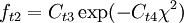
![f_{t1} = C_{t1} g_t \exp\left( -C_{t2} \frac{\omega_t^2}{\Delta U^2} [ d^2 + g^2_t d^2_t] \right)](/W/images/math/9/9/3/993b41d0ba795e0b3877d041c4cff1cb.png)
- d is the distance to the closest surface
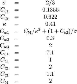
The constants are
Modifications to original model
According to Spalart it is safer to use the following values for the last two constants:

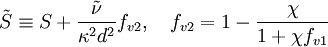
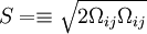
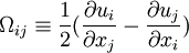
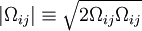
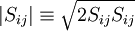
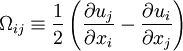
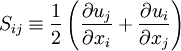
[Dacles-Mariani et. al. 1995] proposed a modification of the model which also accounts for the effect of mean strain rate on turbulence production. This modification instead prescribes:

where

Other models related to the S-A model:
DES (1999) [1]
DDES (2006)
Model for compressible flows
There are two approaches to adapting the model for compressible flows. In the first approach the turbulent dynamic viscosity is computed from

where  is the local density. The convective terms in the equation for are modified to
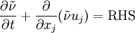
where the right hand side (RHS) is the same as in the original model.
Boundary conditions
Boundary conditions are set by defining values of .
Freestream boundary conditions are discussed in turbulence free-stream boundary conditions.
Walls: 
Outlet: convective outlet.
References
- Dacles-Mariani, J., Zilliac, G. G., Chow, J. S. and Bradshaw, P. (1995), "Numerical/Experimental Study of a Wingtip Vortex in the Near Field", AIAA Journal, 33(9), pp. 1561-1568, 1995.
- Spalart, P. R. and Allmaras, S. R. (1992), "A One-Equation Turbulence Model for Aerodynamic Flows", AIAA Paper 92-0439.
- Spalart, P. R. and Allmaras, S. R. (1994), "A One-Equation Turbulence Model for Aerodynamic Flows", La Recherche Aerospatiale n 1, 5-21.