CFD Online Logo CFD Online URL
www.cfd-online.com
[Sponsors]
Home > Wiki > Explicit nonlinear constitutive relation

Explicit nonlinear constitutive relation

From CFD-Wiki

Jump to: navigation, search
Turbulence modeling
Turbulence
RANS-based turbulence models
  1. Linear eddy viscosity models
    1. Algebraic models
      1. Cebeci-Smith model
      2. Baldwin-Lomax model
      3. Johnson-King model
      4. A roughness-dependent model
    2. One equation models
      1. Prandtl's one-equation model
      2. Baldwin-Barth model
      3. Spalart-Allmaras model
    3. Two equation models
      1. k-epsilon models
        1. Standard k-epsilon model
        2. Realisable k-epsilon model
        3. RNG k-epsilon model
        4. Near-wall treatment
      2. k-omega models
        1. Wilcox's k-omega model
        2. Wilcox's modified k-omega model
        3. SST k-omega model
        4. Near-wall treatment
      3. Realisability issues
        1. Kato-Launder modification
        2. Durbin's realizability constraint
        3. Yap correction
        4. Realisability and Schwarz' inequality
  2. Nonlinear eddy viscosity models
    1. Explicit nonlinear constitutive relation
      1. Cubic k-epsilon
      2. EARSM
    2. v2-f models
      1. \overline{\upsilon^2}-f model
      2. \zeta-f model
  3. Reynolds stress model (RSM)
Large eddy simulation (LES)
  1. Smagorinsky-Lilly model
  2. Dynamic subgrid-scale model
  3. RNG-LES model
  4. Wall-adapting local eddy-viscosity (WALE) model
  5. Kinetic energy subgrid-scale model
  6. Near-wall treatment for LES models
Detached eddy simulation (DES)
Direct numerical simulation (DNS)
Turbulence near-wall modeling
Turbulence free-stream boundary conditions
  1. Turbulence intensity
  2. Turbulence length scale

General Concept

An explicit nonlinear constitutive relation for the Reynolds stresses represents an explicitly-postulated expansion over the linear Boussinesq hypothesis.

One of such explicit and nonlinear expansion over the Boussinesq hypothesis, as proposed by [Wallin & Johansson (2000)], is given by


   \begin{align}
   - \frac{\mathbf{u u}}{k} & + \frac{2}{3} \mathbf{I} = \beta_1 \tilde{\mathbf{S}}
   \\
   & + \beta_2 \left( \tilde{\mathbf{S}}^2 - \frac{II_S}{3} \mathbf{I} \right)
     + \beta_3 \left( \tilde{\mathbf{\Omega}}^2 - \frac{II_\Omega}{3} \mathbf{I} \right)
   \\
   & + \beta_4 \left( \tilde{\mathbf{S}} \tilde{\mathbf{\Omega}} - \tilde{\mathbf{\Omega}} \tilde{\mathbf{S}} \right)
     + \beta_5 \left( \tilde{\mathbf{S}}^2 \tilde{\mathbf{\Omega}} - \tilde{\mathbf{\Omega}} \tilde{\mathbf{S}}^2 \right)
   \\
   & + \beta_6 \left( \tilde{\mathbf{S}} \tilde{\mathbf{\Omega}}^2 + \tilde{\mathbf{\Omega}}^2 \tilde{\mathbf{S}} - \frac{2}{3} IV \mathbf{I} \right)
   \\
   & + \beta_7 \left( \tilde{\mathbf{S}}^2 \tilde{\mathbf{\Omega}}^2 + \tilde{\mathbf{\Omega}}^2 \tilde{\mathbf{S}}^2 - \frac{2}{3} V \mathbf{I} \right)
   \\
   & + \beta_8 \left( \tilde{\mathbf{S}} \tilde{\mathbf{\Omega}} \tilde{\mathbf{S}}^2 + \tilde{\mathbf{S}}^2 \tilde{\mathbf{\Omega}} \tilde{\mathbf{S}} \right)
     + \beta_9 \left( \tilde{\mathbf{\Omega}} \tilde{\mathbf{S}} \tilde{\mathbf{\Omega}}^2 + \tilde{\mathbf{\Omega}}^2 \tilde{\mathbf{S}} \tilde{\mathbf{\Omega}} \right)
   \\
   & + \beta_{10} \left( \tilde{\mathbf{\Omega}} \tilde{\mathbf{S}}^2 \tilde{\mathbf{\Omega}}^2 + \tilde{\mathbf{\Omega}}^2 \tilde{\mathbf{S}}^2 \tilde{\mathbf{\Omega}} \right)
   \end{align}

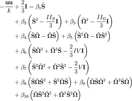
Note that the terms in the first line are exactly the linear relation as expressed by the Boussinesq hypothesis.

Reference

  • Wallin, S., and Johansson, A. V. (2000), "An Explicit Algebraic Reynolds Stress Model for Incompressible and Compressible Turbulent Flows", Journal of Fluid Mechanics, Vol. 403, Jan. 2000, pp. 89–132.


My wiki